In the next section we’ll consider initial value problems
where \(a\), \(b\), and \(c\) are constants and \(f\) is piecewise continuous. In this section we’ll develop procedures for using the table of Laplace transforms to find Laplace transforms of piecewise continuous functions, and to find the piecewise continuous inverses of Laplace transforms.
Example 8.4.1
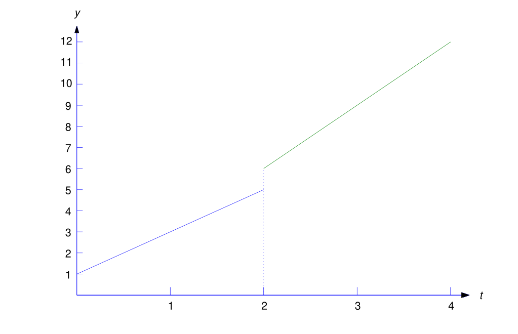
Use the table of Laplace transforms to find the Laplace transform of
(Figure 8.4.1).
Solution Since the formula for \(f\) changes at \(t=2\), we write
To relate the first term to a Laplace transform, we add and subtract
in (8.4.2) to obtain
To relate the last integral to a Laplace transform, we make the change of variable \(x=t-2\) and rewrite the integral as
Since the symbol used for the variable of integration has no effect on the value of a definite integral, we can now replace \(x\) by the more standard \(t\) and write
This and (8.4.3) imply that
Now we can use the table of Laplace transforms to find that
Laplace Transforms of Piecewise Continuous Functions
We’ll now develop the method of Example 8.4.1 into a systematic way to find the Laplace transform of a piecewise continuous function. It is convenient to introduce the unit step function, defined as
Thus, \(u(t)\) “steps” from the constant value \(0\) to the constant value \(1\) at \(t=0\). If we replace \(t\) by \(t-\tau\) in (8.4.4), then
that is, the step now occurs at \(t=\tau\) (Figure 8.4.2).
The step function enables us to represent piecewise continuous functions conveniently. For example, consider the function
where we assume that \(f_0\) and \(f_1\) are defined on \([0,\infty)\), even though they equal \(f\) only on the indicated intervals. This assumption enables us to rewrite (8.4.5) as
To verify this, note that if \(t<t_1\) then \(u(t-t_1)=0\) and (8.4.6) becomes
If \(t\ge t_1\) then \(u(t-t_1)=1\) and (8.4.6) becomes
We need the next theorem to show how (8.4.6) can be used to find \({\cal L}(f)\).
Theorem 8.4.1
Let \(g\) be defined on \([0,\infty).\) Suppose \(\tau\ge0\) and \({\cal L}\left(g(t+\tau)\right)\) exists for \(s>s_0.\) Then \({\cal L}\left(u(t-\tau)g(t)\right)\) exists for \(s>s_0\), and
Proof By definition,
From this and the definition of \(u(t-\tau)\),
The first integral on the right equals zero. Introducing the new variable of integration \(x=t-\tau\) in the second integral yields
Changing the name of the variable of integration in the last integral from \(x\) to \(t\) yields
Example 8.4.2
Find
Solution Here \(\tau=1\) and \(g(t)=t^2+1\), so
Since
Theorem 8.4.1 implies that
Example 8.4.3
Use Theorem 8.4.1 to find the Laplace transform of the function
from Example 8.4.1.
Solution We first write \(f\) in the form (8.4.6) as
Therefore
which is the result obtained in Example 8.4.1.∎
Formula (8.4.6) can be extended to more general piecewise continuous functions. For example, we can write
as
if \(f_0\), \(f_1\), and \(f_2\) are all defined on \([0,\infty)\).
Example 8.4.4
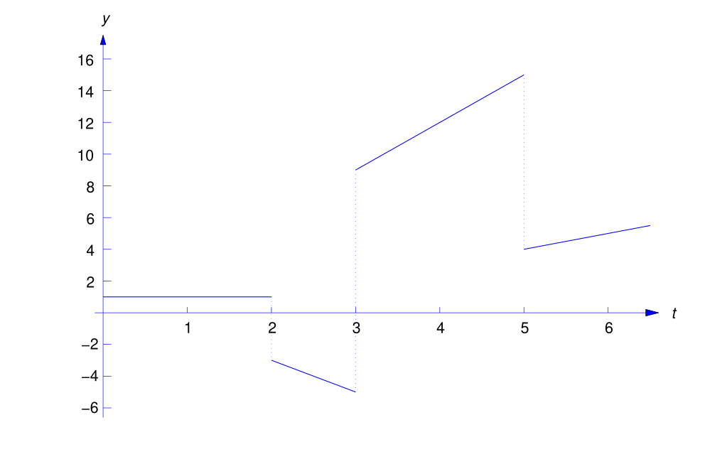
Find the Laplace transform of
(Figure 8.4.3).
Solution In terms of step functions,
or
Now Theorem 8.4.1 implies that
The trigonometric identities
are useful in problems that involve shifting the arguments of trigonometric functions. We’ll use these identities in the next example.
Example 8.4.5
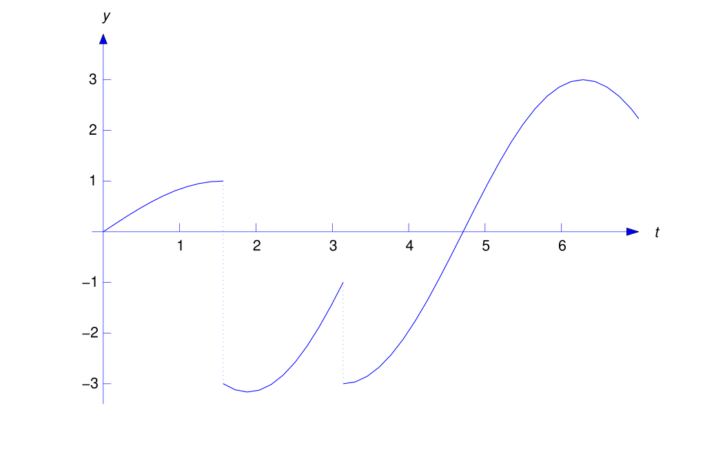
Find the Laplace transform of
(Figure 8.4.4).
Solution In terms of step functions,
Now Theorem 8.4.1 implies that
Since
and
we see from (8.4.11) that
The Second Shifting Theorem
Replacing \(g(t)\) by \(g(t-\tau)\) in Theorem 8.4.1 yields the next theorem.
Theorem 8.4.2
If \(\tau\ge0\) and \({\cal L}(g)\) exists for \(s>s_0\) then \({\cal L}\left(u(t-\tau)g(t-\tau)\right)\) exists for \(s>s_0\) and
or, equivalently,
Remark
Recall that the First Shifting Theorem (Theorem 8.1.3 states that multiplying a function by \(e^{at}\) corresponds to shifting the argument of its transform by \(a\) units. Theorem 8.4.2 states that multiplying a Laplace transform by the exponential \(e^{-\tau s}\) corresponds to shifting the argument of the inverse transform by \(\tau\) units.
Solution To apply (8.4.12) we let \(\tau=2\) and \(G(s)=1/s^2\). Then \(g(t)=t\) and (8.4.12) implies that
Example 8.4.7
Find the inverse Laplace transform \(h\) of
and find distinct formulas for \(h\) on appropriate intervals.
Solution Let
Then
Hence, (8.4.12) and the linearity of \({\cal L}^{-1}\) imply that
which can also be written as
Example 8.4.8
Find the inverse transform of
Solution Let
and
Then
and
Therefore (8.4.12) and the linearity of \({\cal L}^{-1}\) imply that
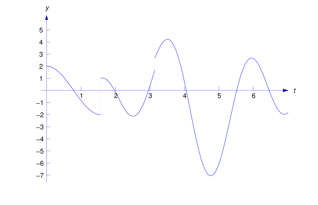
Using the trigonometric identities (8.4.8) and (8.4.9), we can rewrite this as
(Figure 8.4.5).
8.4 Exercises
In Exercises 1–6 find the Laplace transform by the method of Example 8.4.1. Then express the given function \(f\) in terms of unit step functions as in Eqn. (8.4.6), and use Theorem 8.4.1 to find \({\cal L}(f)\). Where indicated by C/G , graph \(f\).
-
\(\dst{f(t)=\left\{\begin{array}{cl} 1,&0 \le t<4,\\[6pt] t,&t\ge4.\end{array}\right.}\)
Show answer
\( 1+u(t-4)(t-1)\); \(\dst{{1\over s}+e^{-4s}\left({1\over s^2}+{3\over s}\right)}\)
-
\(\dst{f(t)=\left\{\begin{array}{cl} t,&0 \le t<1,\\[6pt] 1,&t\ge1.\end{array}\right.}\)
Show answer
\(t+u(t-1)(1-t)\); \(\dst{1-e^{-s}\over s^2}\)
-
C/G \(\dst{f(t)=\left\{\begin{array}{cl} 2t-1,& 0\le t<2,\\[6pt] t,&t\ge2.\end{array}\right.}\)
Show answer
\(2t-1-u(t-2)(t-1)\); \(\dst{\left({2\over s^2}-{1\over s}\right)-e^{-2s}\left({1\over s^2} +{1\over s}\right)}\)
-
C/G \(\dst{f(t)=\left\{\begin{array}{cl}1, &0\le t<1,\\[6pt] t+2,&t\ge1.\end{array}\right.}\)
Show answer
\(1+u(t-1)(t+1)\); \(\dst{{1\over s} +e^{-s}\left({1\over s^2}+{2\over s}\right)}\)
-
\(\dst{f(t)=\left\{\begin{array}{cl} t-1,& 0\le t<2,\\[6pt] 4,&t\ge2.\end{array}\right.}\)
Show answer
\(t-1+u(t-2)(5-t)\); \(\dst{{1\over s^2}-{1\over s}-e^{-2s}\left({1\over s^2}-{3\over s}\right)}\)
-
\(\dst{f(t)=\left\{\begin{array}{cl} t^2,& 0\le t<1,\\[6pt] 0,&t\ge1.\end{array}\right.}\)
Show answer
\(t^2\left(1-u(t-1)\right)\); \(\dst{ {2\over s^3}-e^{-s}\left({2\over s^3}+{2\over s^2}+{1\over s}\right)}\)
In Exercises 7–18 express the given function \(f\) in terms of unit step functions and use Theorem 8.4.1 to find \({\cal L}(f)\). Where indicated by C/G , graph \(f\).
-
\(\dst{f(t)=\left\{\begin{array}{cl} 0, &0\le t<2,\\[6pt] t^2+3t,&t\ge2.\end{array}\right.}\)
Show answer
\(u(t-2)(t^2+3t)\); \(\dst{ e^{-2s}\left({2\over s^3}+{7\over s^2}+{10\over s}\right)}\)
-
\(\dst{f(t)=\left\{\begin{array}{cl} t^2+2, &0\le t<1,\\[6pt] t,&t\ge1.\end{array}\right.}\)
Show answer
\(t^2+2+u(t-1)(t-t^2-2)\); \(\dst{{2\over s^3} +{2\over s}-e^{-s}\left({2\over s^3}+{1\over s^2}+{2 \over s}\right)}\)
-
\(\dst{f(t)=\left\{\begin{array}{cl} te^t,& 0\le t <1,\\[6pt] e^t,&t\ge1.\end{array}\right.}\)
Show answer
\(te^t+u(t-1)(e^t-te^t)\); \(\dst{1-e^{-(s-1)}\over (s-1)^2}\)
-
\(\dst{f(t)=\left\{\begin{array}{cl} e^{\phantom{2}-t}, &0\le t<1,\\[6pt] e^{-2t},&t\ge1.\end{array}\right.}\)
Show answer
\(e^{-t}+u(t-1)(e^{-2t}-e^{-t})\) ; \(\dst{{1-e^{-(s+1)}\over s+1}+{e^{-(s+2)}\over s+2}}\)
-
\(\dst{f(t)=\left\{\begin{array}{cl} -t,&0 \le t<2,\\[6pt] t-4,&2\le t<3,\\[6pt] 1,&t\ge3. \end{array}\right.}\)
Show answer
\(-t+2u(t-2)(t-2)-u(t-3)(t-5)\); \(\dst{-{1\over s^2}+ {2e^{-2s}\over s^2}+e^{-3s}\left({2\over s}-{1\over s^2}\right)}\)
-
\(\dst{f(t)=\left\{\begin{array}{cl} 0,&0 \le t<1,\\[6pt] t,&1\le t<2,\\[6pt] 0,&t\ge2.\end{array}\right.}\)
Show answer
\(\left[u(t-1)-u(t-2)\right]t\) ; \(\dst{ e^{-s}\left({1\over s^2}+{1\over s}\right)-e^{-2s}\left({1\over s^2} +{2\over s}\right)}\)
-
\(\dst{f(t)=\left\{\begin{array}{cl} t,&0 \le t<1,\\[6pt] t^2,&1\le t<2,\\[6pt] 0,&t\ge2. \end{array}\right.}\)
Show answer
\(t+u(t-1)(t^2-t)-u(t-2)t^2\); \(\dst{{1\over s^2}+ e^{-s}\left({2\over s^3}+{1\over s^2}\right) -e^{-2s}\left({2\over s^3}+{4\over s^2}+{4\over s}\right)}\)
-
\(\dst{f(t)=\left\{\begin{array}{cl} t,&0\le t<1,\\[6pt] 2-t,&1\le t<2,\\[6pt] 6,&t > 2. \end{array}\right.}\)
Show answer
\(t+u(t-1)(2-2t)+u(t-2)(4+t)\); \(\dst{{1\over s^2} -2{e^{-s}\over s^2}+e^{-2s}\left({1\over s^2}+{6\over s}\right)}\)
-
C/G \(\dst{f(t)=\left\{\begin{array}{cl} \phantom{2} \sin t,&0\le t<\dst{\pi\over 2},\\[6pt] 2\sin t,& \dst{\pi\over 2}\le t<\pi,\\[6pt]\phantom{2}\cos t, &t\ge\pi.\end{array}\right.}\)
Show answer
\(\dst{\sin t+ u(t-\pi/2)\sin t+u(t-\pi) (\cos t-2\sin t)}\); \(\dst{{1+ e^{-{\pi\over 2}s}s-e^{-\pi s}(s-2)\over s^2+1}}\)
-
C/G \(f(t)=\dst{\left\{\begin{array}{cl}\phantom{-} 2,&0\le t<1,\\[6pt]-2t+2,&1\le t<3,\\[6pt]\phantom{-}3t,&t\ge 3.\end{array}\right.}\)
Show answer
\(\dst{2-2u(t-1)t+u(t-3)(5t-2)}\); \(\dst{{2\over s}-e^{-s}\left({2\over s^2}+{2\over s}\right)+e^{-3s}\left({5\over s^2}+{13\over s}\right)}\)
-
C/G \(f(t)=\dst{\left\{\begin{array}{cl}3,&0\le t<2,\\[6pt]3t+2,&2\le t<4,\\[6pt]4t,&t\ge 4.\end{array}\right.}\)
Show answer
\(\dst{3+u(t-2)(3t-1)+u(t-4)(t-2)}\); \(\dst{{3\over s}+e^{-2s}\left({3\over s^2}+{5\over s}\right)+e^{-4s}\left({1\over s^2}+{2\over s}\right)}\)
-
C/G \(\dst{f(t)=\left\{\begin{array}{ll}(t+1)^2,&0\le t<1, \\[6pt](t+2)^2,&t\ge1.\end{array}\right.}\)
Show answer
\(\dst{(t+1)^2+u(t-1)(2t+3)}\); \(\dst{{2\over s^3 }+{2\over s^2}+{1\over s}+e^{-s}\left({2\over s^2}+{5\over s}\right)}\)
In Exercises 19–28 use Theorem 8.4.2 to express the inverse transforms in terms of step functions, and then find distinct formulas the for inverse transforms on the appropriate intervals, as in Example 8.4.7. Where indicated by C/G , graph the inverse transform.
-
\(\dst{H(s)={e^{-2s}\over s-2}}\)
Show answer
\(u(t-2)e^{2(t-2)}= \dst{\left\{\begin{array}{cl} 0,&0\le t<2, \\[6pt] e^{2(t-2)},&t\ge2.\end{array}\right.}\)
-
\(\dst{H(s)={e^{-s}\over s(s+1)}}\)
Show answer
\(u(t-1)\left(1-e^{-(t-1)}\right)= \dst{\left\{\begin{array}{cl} 0,&0\le t<1,\\[6pt] 1-e^{-(t-1)},&t\ge1.\end{array}\right.}\)
-
C/G \(\dst{H(s)={e^{-s}\over s^3}+ {e^{-2s}\over s^2}}\)
Show answer
\(\dst{u(t-1){(t-1)^2 \over 2}+u(t-2)(t-2)}= \dst{\left\{\begin{array}{cl} 0,&0 \le t< 1,\\[6pt]\dst{(t-1)^2\over 2},&1\le t<2,\\[6pt] \dst{t^2-3\over 2},&t\ge2.\end{array}\right.}\)
-
C/G \(\dst{H(s)=\left({2\over s}+{1\over s^2}\right) +e^{-s}\left({3\over s}-{1\over s^2}\right)+e^{-3s}\left({1\over s}+{1\over s^2}\right)}\)
Show answer
\(2+t+u(t-1)(4-t)+u(t-3)(t-2)= \dst{ \left\{\begin{array}{cl} 2+t,& 0\le t<1,\\[6pt] 6,&1\le t<3,\\[6pt] t+4,&t\ge 3.\end{array}\right.}\)
-
\(\dst{H(s)=\left({5\over s}-{1\over s^2}\right) +e^{-3s}\left({6\over s}+{7\over s^2}\right)+{3e^{-6s}\over s^3}}\)
Show answer
\(\dst{5-t+u(t-3)(7t-15)+ {3\over 2} u(t-6)(t-6)^2}= \dst{\left\{\begin{array}{cl} 5-t,&0\le t<3,\\[6pt] 6t-10,&3\le t<6,\\[6pt] 44-12t+{3\over2}t^2, &t\ge6. \end{array}\right.}\)
-
\(\dst{H(s)={e^{-\pi s} (1-2s)\over s^2+4s+5}}\)
Show answer
\(u(t-\pi)e^{-2(t-\pi)} (2\cos t- 5\sin t)= \dst{\left\{\begin{array}{cl} 0, &0\le t<\pi,\\[6pt] e^{-2(t-\pi)}(2\cos t-5\sin t),&t\ge\pi. \end{array}\right.}\)
-
C/G \(\dst{H(s)=\left({1\over s}-{s\over s^2+1}\right)+e^{-{\pi\over 2}s}\left({3s-1\over s^2+1}\right)}\)
Show answer
\(\dst{1-\cos t+ u(t-\pi/2) (3\sin t+\cos t)}= \dst{\left\{\begin{array}{cl} 1-\cos t,&0\le t<\dst{\pi\over 2},\\[6pt] 1+3\sin t,&t\ge \dst{\pi\over 2}.\end{array}\right.}\)
-
\(\dst{H(s)= e^{-2s}\left[{3(s-3)\over(s+1)(s-2)}-{s+1\over(s-1)(s-2)}\right]}\)
Show answer
\(\dst{u(t-2)\left (4e^{-(t-2)}-4e^{2(t-2)}+2e^{(t-2)}\right)}= \dst{\left\{\begin{array}{cl} 0,&0\le t<2,\\[6pt]4e^{-(t-2)}-4e^{2(t-2)}+2e^{(t-2)},&t\ge 2.\end{array}\right.}\)
-
\(\dst{H(s)={1\over s}+{1\over s^2}+e^{-s}\left({3\over s}+{2\over s^2}\right) +e^{-3s}\left({4\over s}+{3\over s^2}\right)}\)
Show answer
\(\dst{1+t+u(t-1)(2t+1)+u(t-3)(3t-5)}= \dst{ \left\{\begin{array}{cl} t+1,&0\le t<1,\\[6pt] 3t+2,&1\le t<3,\\[6pt]6t-3,&t\ge3.\end{array}\right.}\)
-
\(\dst{H(s)={1\over s}-{2\over s^3}+e^{-2s}\left({3\over s}-{1\over s^3}\right) +{e^{-4s}\over s^2}}\)
Show answer
\(\dst{1-t^2+u(t-2)\left(-{t^2\over2}+2t+1\right) +u(t-4)(t-4)}= \dst{\left\{\begin{array}{cl} 1-t^2,&0\le t<2\\[6pt]-\dst{3t^2\over2} +2t+2,&2\le t<4,\\[6pt]-\dst{3t^2\over2}+3t-2,&t\ge 4.\end{array}\right.}\)
-
Find \({\cal L}\left(u(t-\tau)\right)\).
Show answer
\(\dst{e^{-\tau s}\over s}\)
-
Let \(\{t_m\}_{m=0}^\infty\) be a sequence of points such that \(t_0=0\), \(t_{m+1}>t_m\), and \(\lim_{m\to\infty}t_m=\infty\). For each nonnegative integer \(m\), let \(f_m\) be continuous on \([t_m,\infty)\), and let \(f\) be defined on \([0,\infty)\) by
\[ f(t)=f_m(t),\,t_m\le t<t_{m+1}\quad (m=0,1,\dots). \]Show that \(f\) is piecewise continuous on \([0,\infty)\) and that it has the step function representation
\[ f(t)=f_0(t)+\sum_{m=1}^\infty u(t-t_m)\left(f_m(t)-f_{m-1}(t)\right),\, 0\le t<\infty. \]How do we know that the series on the right converges for all \(t\) in \([0,\infty)\)?
Show answer
For each \(t\) only finitely many terms are nonzero.
-
In addition to the assumptions of Exercise 30, assume that
\[ |f_m(t)|\le Me^{s_0t},\,t\ge t_m,\,m=0,1,\dots, \tag*{\rm (A)} \]and that the series
\[ \sum_{m=0}^\infty e^{-\rho t_m} \tag*{\rm (B)} \]converges for some \(\rho>0\). Using the steps listed below, show that \({\cal L}(f)\) is defined for \(s>s_0\) and
\[ {\cal L}(f)={\cal L}(f_0)+\sum_{m=1}^\infty e^{-st_m}{\cal L}(g_m) \tag*{\rm (C)} \]for \(s>s_0+\rho\), where
\[ g_m(t)=f_m(t+t_m)-f_{m-1}(t+t_m). \]Use (A) and Theorem 8.1.6 to show that
\[ {\cal L}(f)=\sum_{m=0}^\infty\int_{t_m}^{t_{m+1}}e^{-st}f_m(t)\,dt \tag*{\rm (D)} \]is defined for \(s>s_0\).
Show that (D) can be rewritten as
\[ {\cal L}(f)=\sum_{m=0}^\infty\left(\int_{t_m}^\infty e^{-st}f_m(t)\,dt -\int_{t_{m+1}}^\infty e^{-st}f_m(t)\,dt\right). \tag*{\rm (E)} \]Use (A), the assumed convergence of (B), and the comparison test to show that the series
\[ \sum_{m=0}^\infty\int_{t_m}^\infty e^{-st}f_m(t)\,dt\mbox{\quad and \quad} \sum_{m=0}^\infty\int_{t_{m+1}}^\infty e^{-st}f_m(t)\,dt \]both converge (absolutely) if \(s>s_0+\rho\).
Show that (E) can be rewritten as
\[ {\cal L}(f)={\cal L}(f_0)+\sum_{m=1}^\infty\int_{t_m}^\infty e^{-st} \left(f_m(t)-f_{m-1}(t)\right)\,dt \]if \(s>s_0+\rho\).
Complete the proof of (C).
-
Suppose \(\{t_m\}_{m=0}^\infty\) and \(\{f_m\}_{m=0}^\infty\) satisfy the assumptions of Exercises 30 and 31, and there’s a positive constant \(K\) such that \(t_m\ge Km\) for \(m\) sufficiently large. Show that the series (B) of Exercise 31 converges for any \(\rho>0\), and conclude from this that (C) of Exercise 31 holds for \(s>s_0\).
In Exercises 33–36 find the step function representation of \(f\) and use the result of Exercise 32 to find \({\cal L}(f)\). Hint: You will need formulas related to the formula for the sum of a geometric series.
-
\(f(t)=m+1,\,m\le t<m+1\; (m=0,1,2,\dots)\)
Show answer
\(\dst{1+\sum_{m=1}^\infty u(t-m);\; {1\over s(1-e^{-s})}}\)
-
\(f(t)=(-1)^m,\,m\le t<m+1\; (m=0,1,2,\dots)\)
Show answer
\(\dst{1+2\sum_{m=1}^\infty (-1)^mu(t-m);\; {1\over s};\; {1-e^{-s}\over 1+e^{-s}}}\)
-
\(f(t)=(m+1)^2,\,m\le t<m+1\; (m=0,1,2,\dots)\)
Show answer
\(\dst{1+\sum_{m=1}^\infty(2m+1)u(t-m);\; {e^{-s}(1+e^{-s})\over s(1-e^{-s})^2}}\)
-
\(f(t)=(-1)^mm,\,m\le t<m+1\; (m=0,1,2,\dots)\)
Show answer
\(\dst{\sum_{m=1}^\infty(-1)^m(2m-1)u(t-m);\; {1\over s}{(1-e^s)\over(1+e^s)^2}}\)