Definition of the Laplace Transform
To define the Laplace transform, we first recall the definition of an improper integral. If \(g\) is integrable over the interval \([a,T]\) for every \(T>a\), then the improper integral of \(g\) over \([a,\infty)\) is defined as
We say that the improper integral converges if the limit in (8.1.1) exists; otherwise, we say that the improper integral diverges or does not exist. Here’s the definition of the Laplace transform of a function \(f\).
Definition 8.1.1
Let \(f\) be defined for \(t\ge0\) and let \(s\) be a real number\(.\) Then the Laplace transform of \(f\) is the function \(F\) defined by
for those values of \(s\) for which the improper integral converges\(.\)
It is important to keep in mind that the variable of integration in (8.1.2) is \(t\), while \(s\) is a parameter independent of \(t\). We use \(t\) as the independent variable for \(f\) because in applications the Laplace transform is usually applied to functions of time.
The Laplace transform can be viewed as an operator \({\cal L}\) that transforms the function \(f=f(t)\) into the function \(F=F(s)\). Thus, (8.1.2) can be expressed as
The functions \(f\) and \(F\) form a transform pair, which we’ll sometimes denote by
It can be shown that if \(F(s)\) is defined for \(s=s_0\) then it’s defined for all \(s>s_0\) (Exercise 14(b)).
Computation of Some Simple Laplace Transforms
Example 8.1.1
Find the Laplace transform of \(f(t)=1\).
Solution From (8.1.2) with \(f(t)=1\),
If \(s\ne 0\) then
Therefore
If \(s=0\) the integrand reduces to the constant \(1\), and
Therefore \(F(0)\) is undefined, and
This result can be written in operator notation as
or as the transform pair
Remark
It is convenient to combine the steps of integrating from \(0\) to \(T\) and letting \(T\to\infty\). Therefore, instead of writing (8.1.3) and (8.1.4) as separate steps we write
We’ll follow this practice throughout this chapter.
Example 8.1.2
Find the Laplace transform of \(f(t)=t\).
Solution From (8.1.2) with \(f(t)=t\),
If \(s\ne0\), integrating by parts yields
If \(s=0\), the integral in (8.1.5) becomes
Therefore \(F(0)\) is undefined and
This result can also be written as
or as the transform pair
Example 8.1.3
Find the Laplace transform of \(f(t)=e^{at}\), where \(a\) is a constant.
Solution From (8.1.2) with \(f(t)=e^{at}\),
Combining the exponentials yields
However, we know from Example 8.1.1 that
Replacing \(s\) by \(s-a\) here shows that
This can also be written as
Example 8.1.4
Find the Laplace transforms of \(f(t)=\sin\omega t\) and \(g(t)=\cos\omega t\), where \(\omega\) is a constant.
Solution Define
and
If \(s>0\), integrating (8.1.6) by parts yields
so
If \(s>0\), integrating (8.1.7) by parts yields
so
Now substitute from (8.1.8) into this to obtain
Solving this for \(G(s)\) yields
This and (8.1.8) imply that
Tables of Laplace transforms
Extensive tables of Laplace transforms have been compiled and are commonly used in applications. The brief table of Laplace transforms in the Appendix will be adequate for our purposes.
Example 8.1.5
Use the table of Laplace transforms to find \({\cal L}(t^3e^{4t})\).
Solution The table includes the transform pair
Setting \(n=3\) and \(a=4\) here yields
We’ll sometimes write Laplace transforms of specific functions without explicitly stating how they are obtained. In such cases you should refer to the table of Laplace transforms.
Linearity of the Laplace Transform
The next theorem presents an important property of the Laplace transform.
Theorem 8.1.2
Suppose \({\cal L}(f_i)\) is defined for \(s>s_i,\) \(1\le i\le n).\) Let \(s_0\) be the largest of the numbers \(s_1\), \(s_{2},\) …,\(s_n,\) and let \(c_1\), \(c_2\),…, \(c_n\) be constants\(.\) Then
Proof We give the proof for the case where \(n=2\). If \(s>s_0\) then
Example 8.1.6
Use Theorem 8.1.2 and the known Laplace transform
to find \({\cal L}(\cosh bt)\,(b\ne0)\).
Solution By definition,
Therefore
where the first transform on the right is defined for \(s>b\) and the second for \(s>-b\); hence, both are defined for \(s>|b|\). Simplifying the last expression in (8.1.9) yields
The First Shifting Theorem
The next theorem enables us to start with known transform pairs and derive others. (For other results of this kind, see Exercises 6 and 13.)
Theorem 8.1.3
If
is the Laplace transform of \(f(t)\) for \(s>s_0\), then \(F(s-a)\) is the Laplace transform of \(e^{at}f(t)\) for \(s >s_0+a\).
Proof. Replacing \(s\) by \(s-a\) in (8.1.10) yields
if \(s-a>s_0\); that is, if \(s>s_0+a\). However, (8.1.11) can be rewritten as
which implies the conclusion.
Example 8.1.7
Use Theorem 8.1.3 and the known Laplace transforms of \(1\), \(t\), \(\cos\omega t\), and \(\sin\omega t\) to find
Solution In the following table the known transform pairs are listed on the left and the required transform pairs listed on the right are obtained by applying Theorem 8.1.3.
| \(f(t)\leftrightarrow F(s)\) | \(e^{at}f(t)\leftrightarrow F(s-a)\) |
| \(1\leftrightarrow\dst{1\over s},\quad s>0\) | \(e^{at}\leftrightarrow\dst{1\over(s-a)},\quad s>a\) |
| \(t\leftrightarrow\dst{{1\over s^2}},\quad s>0\) | \(te^{at}\leftrightarrow\dst{{1\over(s-a)^2}},\quad s>a\) |
| \(\sin\omega t\leftrightarrow\dst{{\omega\over s^2+\omega^2}},\quad s>0\) | \(e^{\lambda t}\sin\omega t\leftrightarrow\dst{{\omega\over (s-\lambda)^2+\omega^2}},\,s>\lambda\) |
| \(\cos\omega t\leftrightarrow\dst{{s\over s^2+\omega^2}},\quad s>0\) | \(e^{\lambda t}\sin\omega t\leftrightarrow\dst{{s-\lambda\over (s-\lambda)^2+\omega^2}},\,s>\lambda\) |
Existence of Laplace Transforms
Not every function has a Laplace transform. For example, it can be shown (Exercise 3) that
for every real number \(s\). Hence, the function \(f(t)=e^{t^2}\) does not have a Laplace transform.
Our next objective is to establish conditions that ensure the existence of the Laplace transform of a function. We first review some relevant definitions from calculus.
Recall that a limit
exists if and only if the one-sided limits
both exist and are equal; in this case,
Recall also that \(f\) is continuous at a point \(t_0\) in an open interval \((a,b)\) if and only if
which is equivalent to
For simplicity, we define
so (8.1.12) can be expressed as
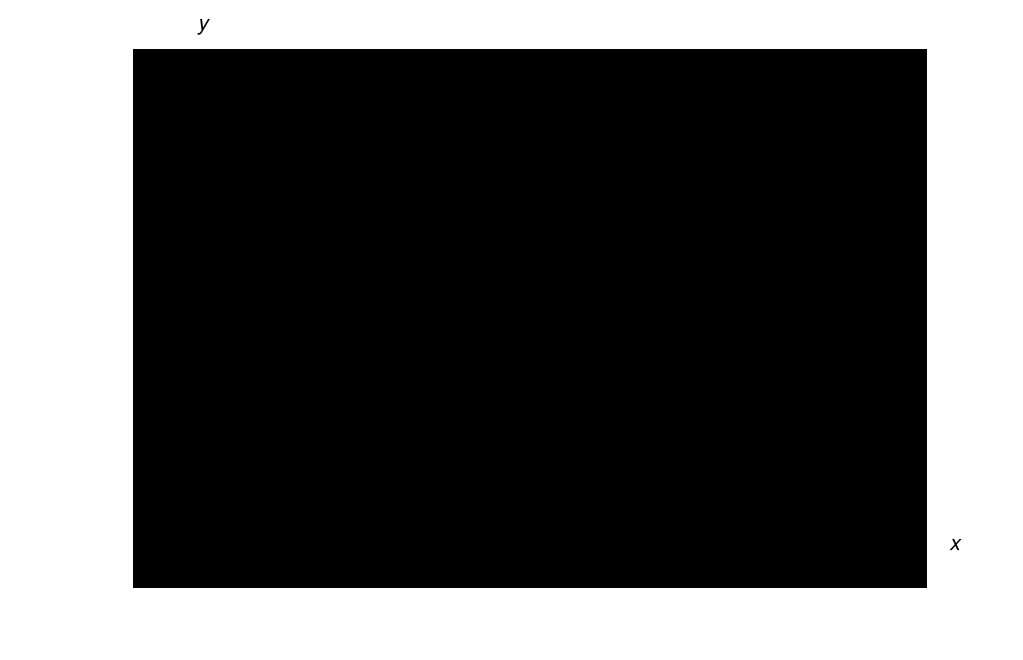
If \(f(t_0+)\) and \(f(t_0-)\) have finite but distinct values, we say that \(f\) has a jump discontinuity at \(t_0\), and
is called the jump in \(f\) at \(t_0\) (Figure 8.1.1).
If \(f(t_0+)\) and \(f(t_0-)\) are finite and equal, but either \(f\) isn’t defined at \(t_0\) or it’s defined but
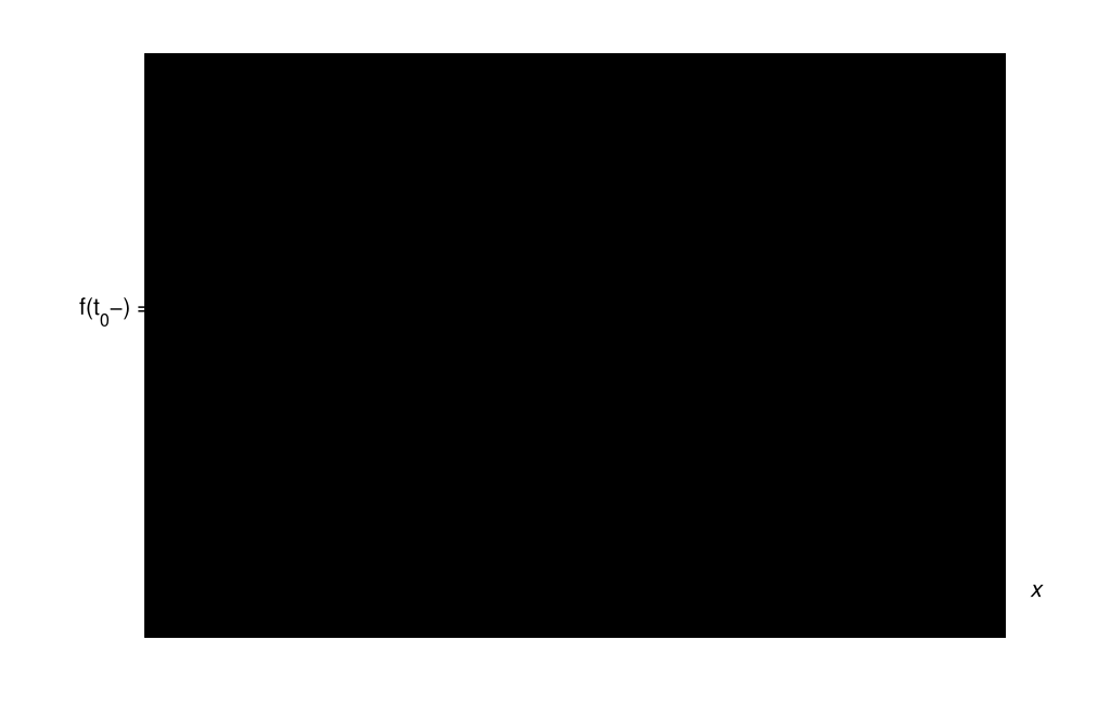
we say that \(f\) has a removable discontinuity at \(t_0\) (Figure 8.1.2). This terminolgy is appropriate since a function \(f\) with a removable discontinuity at \(t_0\) can be made continuous at \(t_0\) by defining (or redefining)
![A piecewise continuous function on [a,b]](/differentialEquations/figures/fig080103.svg)
Remark
We know from calculus that a definite integral isn’t affected by changing the values of its integrand at isolated points. Therefore, redefining a function \(f\) to make it continuous at removable discontinuities does not change \({\cal L}(f)\).
Definition 8.1.4
A function \(f\) is said to be piecewise continuous on a finite closed interval \([0,T]\) if \(f(0+)\) and \(f(T-)\) are finite and \(f\) is continuous on the open interval \((0,T)\) except possibly at finitely many points, where \(f\) may have jump discontinuities or removable discontinuities.
A function \(f\) is said to be piecewise continuous on the infinite interval \([0,\infty)\) if it’s piecewise continuous on \([0,T]\) for every \(T>0\).
Figure 8.1.3 shows the graph of a typical piecewise continuous function.
It is shown in calculus that if a function is piecewise continuous on a finite closed interval then it’s integrable on that interval. But if \(f\) is piecewise continuous on \([0,\infty)\), then so is \(e^{-st}f (t)\), and therefore
exists for every \(T>0\). However, piecewise continuity alone does not guarantee that the improper integral
converges for \(s\) in some interval \((s_0,\infty)\). For example, we noted earlier that (8.1.13) diverges for all \(s\) if \(f(t)=e^{t^2}\). Stated informally, this occurs because \(e^{t^2}\) increases too rapidly as \(t\to\infty\). The next definition provides a constraint on the growth of a function that guarantees convergence of its Laplace transform for \(s\) in some interval \((s_0,\infty)\) .
Definition 8.1.5
A function \(f\) is said to be of exponential order \(s_0\) if there are constants \(M\) and \(t_0\) such that
In situations where the specific value of \(s_0\) is irrelevant we say simply that \(f\) is of exponential order.
The next theorem gives useful sufficient conditions for a function \(f\) to have a Laplace transform. The proof is sketched in Exercise 10.
Theorem 8.1.6
If \(f\) is piecewise continuous on \([0,\infty)\) and of exponential order \(s_0,\) then \({\cal L}(f)\) is defined for \(s>s_0\).
Remark
We emphasize that the conditions of Theorem 8.1.6 are sufficient, but not necessary, for \(f\) to have a Laplace transform. For example, Exercise 14(c) shows that \(f\) may have a Laplace transform even though \(f\) isn’t of exponential order.
Example 8.1.8
If \(f\) is bounded on some interval \([t_0,\infty)\), say
then (8.1.14) holds with \(s_0=0\), so \(f\) is of exponential order zero. Thus, for example, \(\sin\omega t\) and \(\cos \omega t\) are of exponential order zero, and Theorem 8.1.6 implies that \({\cal L}(\sin\omega t)\) and \({\cal L}(\cos \omega t)\) exist for \(s>0\). This is consistent with the conclusion of Example 8.1.4.
Example 8.1.9
It can be shown that if \(\lim_{t\to\infty}e^{-s_0t}f(t)\) exists and is finite then \(f\) is of exponential order \(s_0\) (Exercise 9). If \(\alpha\) is any real number and \(s_0>0\) then \(f(t)=t^\alpha\) is of exponential order \(s_0\), since
by L’Hôpital’s rule. If \(\alpha\ge 0\), \(f\) is also continuous on \([0,\infty)\). Therefore Exercise 9 and Theorem 8.1.6 imply that \({\cal L}(t^\alpha)\) exists for \(s\ge s_0\). However, since \(s_0\) is an arbitrary positive number, this really implies that \({\cal L}(t^\alpha)\) exists for all \(s>0\). This is consistent with the results of Example 8.1.2 and Exercises 6 and 8.
Example 8.1.10
Find the Laplace transform of the piecewise continuous function
Solution Since \(f\) is defined by different formulas on \([0,1)\) and \([1,\infty)\), we write
Since
and
it follows that
This is consistent with Theorem 8.1.6, since
and therefore \(f\) is of exponential order \(s_0=-1\).
Remark
In Section 8.4 we’ll develop a more efficient method for finding Laplace transforms of piecewise continuous functions.
Example 8.1.11
We stated earlier that
for all \(s\), so Theorem 8.1.6 implies that \(f(t)=e^{t^2}\) is not of exponential order, since
so
for sufficiently large values of \(t\), for any choice of \(M\) and \(s_{0}\) (Exercise 3).
8.1 Exercises
-
Find the Laplace transforms of the following functions by evaluating the integral \(F(s)=\int_0^\infty e^{-st} f(t)\,dt\).
(a) \(t\) (b) \(te^{-t}\) (c) \(\sinh bt\) (d) \(e^{2t}-3e^t\) (e) \(t^2\) Show answer
(a) \(\dst{1\over s^2}\) (b) \(\dst{1\over(s+1)^2}\) (c) \(\dst{b\over s^2-b^2}\) (d) \(\dst{-2s+5\over(s-1)(s-2)}\) (e) \(\dst{2\over s^3}\)
-
Use the table of Laplace transforms to find the Laplace transforms of the following functions.
(a) \(\cosh t\sin t\) (b) \(\sin^2t\) (c) \(\cos^2 2t\) (d) \(\cosh^2 t\) (e) \(t\sinh 2t\) (f) \(\sin t\cos t\) (g) \(\dst{\sin\left(t+{\pi\over 4}\right)}\) (h) \(\cos 2t -\cos 3t\) (i) \(\sin 2t +\cos 4t\) Show answer
(a) \(\dst{{s^2+2\over\left[(s-1)^2+1\right] \left[(s+1)^2 +1\right]}}\) (b) \(\dst{2\over s(s^2+4)}\) (c) \(\dst{s^2+8\over s(s^2+16)}\) (d) \(\dst{s^2-2\over s(s^2-4)}\)
(e) \(\dst{4s\over(s^2-4)^2}\) (f) \(\dst{1\over s^2+4}\) (g) \(\dst{{1\over\sqrt{2}}\,{s+1\over s^2+1}}\) (h) \(\dst{5s\over(s^2+4)(s^2+9)}\) (i) \(\dst{{s^3+2s^2+4s+32\over (s^2+4)(s^2+16)}}\)
-
Show that
\[ \int_0^\infty e^{-st}e^{t^2} dt=\infty \]for every real number \(s\).
-
Graph the following piecewise continuous functions and evaluate \(f(t+)\), \(f(t-)\), and \(f(t)\) at each point of discontinuity.
(a) \(f(t)=\left\{\begin{array}{cl} -t, & 0\le t<2,\\ t-4, & 2\le t<3,\\ 1, & t\ge 3.\end{array}\right.\) (b) \(f(t)=\left\{\begin{array}{cl} t^2+2, & 0 \le t<1,\\4, & t=1,\\ t, & t> 1.\end{array}\right.\) (c) \(f(t)=\left\{\begin{array}{rl} \sin t, & 0\le t<\pi/ 2,\\ 2\sin t, &\pi/ 2 \le t<\pi,\\ \cos t, & t\ge\pi.\end{array}\right.\) (d) \(f(t)=\left\{\begin{array}{cl}t, & 0\le t<1,\\ 2, & t=1,\\ 2-t, & 1 \le t<2,\\ 3, & t=2,\\ 6, & t> 2.\end{array}\right.\) Show answer
(a) \(\dst{f(3-)=-1,\,f(3)=f(3+)=1}\) (b) \(\dst{f(1-)=3,\,f(1)=4,\,f(1+)=1}\)
(c) \(\dst{f\left({\pi\over2}-\right)=1,\, f\left({\pi\over2}\right)=f\left({\pi\over2}+\right)=2,\, f(\pi-)=0,\,f(\pi)=f(\pi+)=-1}\)
(d) \(\dst{f(1-)=1,\,f(1)=2,\,f(1+)=1,\,f(2-)=0,\,f(2)=3,\,f(2+)=6}\)
-
Find the Laplace transform:
(a) \(f(t)=\left\{\begin{array}{rl} e^{-t}, & 0\le t<1,\\ e^{-2t}, & t\ge 1.\end{array}\right.\) (b) \(f(t)=\left\{\begin{array}{rl} 1, & 0\le t< 4,\\ t, & t\ge 4.\end{array}\right.\) (c) \(f(t)=\left\{\begin{array}{rl} t, & 0\le t<1,\\ 1, & t\ge 1.\end{array}\right.\) (d) \(f(t)=\left\{\begin{array}{rl} te^t, & 0\le t<1,\\\phantom{t} e^t, & t\ge 1.\end{array}\right.\) Show answer
(a) \(\dst{{1 -e^{-(s+1)}\over s+1}+ {e^{-(s+2)}\over s+2}}\) (b) \(\dst{{1\over s}+e^{-4s}\left({1\over s^2}+{3\over s}\right)}\) (c) \(\dst{1-e^{-s}\over s^2}\) (d) \(\dst{1-e^{-(s-1)}\over(s-1)^2}\)
-
Prove that if \(f(t)\leftrightarrow F(s)\) then \(t^kf(t)\leftrightarrow (-1)^kF^{(k)}(s)\). Hint: Assume that it’s permissible to differentiate the integral \(\int_0^\infty e^{-st}f(t)\,dt\) with respect to \(s\) under the integral sign.
-
Use the known Laplace transforms
\[ {\cal L}(e^{\lambda t}\sin\omega t)={\omega\over(s-\lambda)^2+\omega^2} \quad\mbox{and }\quad {\cal L}(e^{\lambda t}\cos\omega t)={s-\lambda\over(s-\lambda)^2+\omega^2} \]and the result of Exercise 6 to find \({\cal L}(te^{\lambda t}\cos\omega t)\) and \({\cal L}(te^{\lambda t}\sin\omega t)\).
Show answer
\(\dst{{\cal L}(e^{\lambda t}\cos\omega t)={(s-\lambda)^2 - \omega^2\over\left((s-\lambda)^2+\omega^2\right)^2}\; {\cal L}(e^{\lambda t}\sin\omega t)= {2\omega(s-\lambda)\over\left((s-\lambda)^2+\omega^2\right)^2}}\)
-
Use the known Laplace transform \({\cal L}(1)=1/s\) and the result of Exercise 6 to show that
\[ {\cal L}(t^n)={n!\over s^{n+1}},\quad n=\mbox{ integer}. \] -
Show that if \(\lim_{t\to\infty} e^{-s_0t} f(t)\) exists and is finite then \(f\) is of exponential order \(s_0\).
Show that if \(f\) is of exponential order \(s_0\) then \(\lim_{t \to\infty} e^{-st} f(t)=0\) for all \(s>s_0\).
Show that if \(f\) is of exponential order \(s_0\) and \(g(t)=f(t+\tau)\) where \(\tau>0\), then \(g\) is also of exponential order \(s_0\).
-
Recall the next theorem from calculus.
Theorem A. Let \(g\) be integrable on \([0,T]\) for every \(T>0.\) Suppose there’s a function \(w\) defined on some interval \([\tau,\infty)\) (with \(\tau\ge 0\)) such that \(|g(t)|\le w(t)\) for \(t\ge\tau\) and \(\int^\infty_\tau w(t)\,dt\) converges. Then \(\int_0^\infty g(t)\,dt\) converges.
Use Theorem A to show that if \(f\) is piecewise continuous on \([0,\infty)\) and of exponential order \(s_0\), then \(f\) has a Laplace transform \(F(s)\) defined for \(s>s_0\).
-
Prove: If \(f\) is piecewise continuous and of exponential order then \(\lim_{s\to\infty}F(s)~=~0\).
-
Prove: If \(f\) is continuous on \([0,\infty)\) and of exponential order \(s_0>0\), then
\[ {\cal L}\left(\int^t_0 f(\tau)\,d\tau\right)={1\over s} {\cal L} (f), \quad s>s_0. \]Hint: Use integration by parts to evaluate the transform on the left.
-
Suppose \(f\) is piecewise continuous and of exponential order, and that \(\lim_{t\to 0+} f(t)/t\) exists. Show that
\[ {\cal L}\left({f(t)\over t}\right)=\int^\infty_s F(r)\,dr. \]Hint: Use the results of Exercises \(6\) and \(11\).
-
Suppose \(f\) is piecewise continuous on \([0,\infty)\).
Prove: If the integral \(g(t)=\int^t_0 e^{-s_0\tau} f(\tau)\,d\tau\) satisfies the inequality \(|g(t)|\le M\; (t\ge 0)\), then \(f\) has a Laplace transform \(F(s)\) defined for \(s>s_0\).
Hint
Use integration by parts to show that
\[ \int_0^T e^{-st}f(t)\,dt = e^{-(s-s_0)T}g(T) +(s-s_0)\int_0^Te^{-(s-s_0)t}g(t)\,dt. \]Show that if \({\cal L}(f)\) exists for \(s=s_0\) then it exists for \(s>s_0\). Show that the function
\[ f(t)=te^{t^2}\cos(e^{t^2}) \]has a Laplace transform defined for \(s>0\), even though \(f\) isn’t of exponential order.
Show that the function
\[ f(t)=te^{t^2}\cos(e^{t^2}) \]has a Laplace transform defined for \(s>0\), even though \(f\) isn’t of exponential order.
-
Use the table of Laplace transforms and the result of Exercise 13 to find the Laplace transforms of the following functions.
(a) \(\dst{{\sin\omega t\over t}\quad(\omega>0)}\) (b) \(\dst{{\cos\omega t-1\over t}}\quad (\omega>0)\) (c) \(\dst{{e^{at}-e^{bt}\over t}}\) (d) \(\dst{{\cosh t-1\over t}}\) (e) \(\dst{{\sinh^2 t\over t}}\) Show answer
(a) \(\dst{\tan^{-1} {\omega\over s},\quad s>0}\) (b) \(\dst{{1\over 2}\ln{s^2\over s^2+\omega^2},\quad s>0}\) (c) \(\dst{{\ln{s-b\over s-a},\quad s>\max (a,b)}}\)
(d) \(\dst{{1\over 2}\ln{s^2\over s^2-1},\quad s>1}\) (e) \(\dst{{1\over 4}\ln{s^2\over s^2-4},\quad s>2}\)
-
The gamma function is defined by
\[ \Gamma (\alpha)=\int_0^\infty x^{\alpha-1}e^{-x}\,dx, \]which can be shown to converge if \(\alpha>0\).
Use integration by parts to show that
\[ \Gamma (\alpha+1)=\alpha\Gamma (\alpha),\quad\alpha>0. \]Show that \(\Gamma(n+1)=n!\) if \(n=1\), \(2\), \(3\),….
From (b) and the table of Laplace transforms,
\[ {\cal L}(t^\alpha)={\Gamma (\alpha+1)\over s^{\alpha+1}},\quad s>0, \]if \(\alpha\) is a nonnegative integer. Show that this formula is valid for any \(\alpha>-1\). Hint: Change the variable of integration in the integral for \(\Gamma (\alpha+1)\).
-
Suppose \(f\) is continuous on \([0, T]\) and \(f(t+T)=f(t)\) for all \(t\ge 0\). (We say in this case that \(f\) is periodic with period \(T\).)
Conclude from Theorem 8.1.6 that the Laplace transform of \(f\) is defined for \(s>0\). Hint: Since \(f\) is continuous on \([0,T]\) and periodic with period \(T\), it’s bounded on \([0,\infty)\).
(b) Show that
\[ F(s)={1\over 1-e^{-sT}}\int_0^T e^{-st}f(t)\,dt,\quad s>0. \]Hint
Write
\[ F(s)=\sum^\infty_{n=0}\int^{(n+1)T}_{nT}e^{-st} f(t)\,dt. \]Then show that
\[ \int^{(n+1)T}_{nT} e^{-st}f(t)\,dt=e^{-nsT}\int_0^T e^{-st}f(t)\,dt, \]and recall the formula for the sum of a geometric series.
-
Use the formula given in Exercise 17(b) to find the Laplace transforms of the given periodic functions:
\(\dst{f(t)=\left\{\begin{array}{cl} t, & 0\le t<1,\\ 2-t, & 1\le t<2,\end{array}\right.\hskip30pt f(t+2)=f(t), \quad t\ge 0}\)
\(\dst{f(t)=\left\{\begin{array}{rl}1, & 0\le t<{1\over 2},\\ -1, & {1\over 2}\le t<1,\end{array}\right. \hskip30pt f(t+1)=f(t),\quad t\ge 0}\)
\(f(t)=|\sin t|\)
\(\dst{f(t)=\left\{\begin{array}{cl}\sin t, & 0\le t< \pi, \\ 0, &\pi\le t<2\pi,\end{array}\right.\hskip30pt f(t+2\pi)=f(t)}\)
Show answer
(a) \(\dst{1\over s^2}\tanh{s\over 2}\) (b) \(\dst{1\over s}\tanh{s\over 4}\) (c) \(\dst{{1\over s^2+1}\coth {\pi s\over 2}}\) (d) \(\dst{1\over(s^2+1)(1-e^{-\pi s})}\)