8.3 Solution of Initial Value Problems

Laplace Transforms of Derivatives

In the rest of this chapter we’ll use the Laplace transform to solve initial value problems for constant coefficient second order equations. To do this, we must know how the Laplace transform of \(f'\) is related to the Laplace transform of \(f\). The next theorem answers this question.

Theorem 8.3.1

Suppose \(f\) is continuous on \([0,\infty)\) and of exponential order \(s_0\), and \(f'\) is piecewise continuous on \([0,\infty).\) Then \(f\) and \(f'\) have Laplace transforms for \(s > s_0,\) and

\begin{equation} {\cal L}(f')=s {\cal L}(f)-f(0). \tag{8.3.1}\end{equation}

Proof

We know from Theorem 8.1.6 that \({\cal L}(f)\) is defined for \(s>s_0\). We first consider the case where \(f'\) is continuous on \([0,\infty)\). Integration by parts yields

\begin{equation} \begin{array}{ccl} \dst\int^T_0 e^{-st}f'(t)\,dt &=&\dst e^{-st}f(t)\Big|^T_0+s \dst \int^T_0e^{-st}f(t)\,dt\\ &=& \dst e^{-sT}f(T)-f(0)+s\int^T_0 e^{-st}f(t)\,dt \end{array} \tag{8.3.2}\end{equation}

for any \(T>0\). Since \(f\) is of exponential order \(s_0\), \(\lim_{T\to \infty}e^{-sT}f(T)=0\) and the last integral in (8.3.2) converges as \(T\to\infty\) if \(s> s_0\). Therefore

\begin{eqnarray*} \int^\infty_0 e^{-st}f'(t)\,dt&=&-f(0)+s\int^\infty_0 e^{-st}f(t)\,dt \\ &=&-f(0)+s{\cal L}(f), \end{eqnarray*}

which proves (8.3.1). Now suppose \(T>0\) and \(f'\) is only piecewise continuous on \([0,T]\), with discontinuities at \(t_1 < t_2 <\cdots < t_{n-1}\). For convenience, let \(t_0=0\) and \(t_n=T\). Integrating by parts yields

\begin{eqnarray*} \int^{t_i}_{t_{i-1}}e^{-st}f'(t)\,dt &=& e^{-st}f(t)\Big|^{t_i}_{t_{i-1}}+s\int^{t_i}_{t_{i-1}}e^{-st}f(t)\,dt \\ &=& e^{-st_i} f(t_i)- e^{-st_{i-1}}f(t_{i-1})+s\int^{t_i}_{t_{i-1}}e^{-st}f(t)\,dt. \end{eqnarray*}

Summing both sides of this equation from \(i=1\) to \(n\) and noting that

\[ \left(e^{-st_1}f(t_1)-e^{-st_0}f(t_0)\right)+\left(e^{-st_2} f(t_2)-e^{-st_1}f(t_1)\right) +\cdots+\left(e^{-st_N}f(t_N)-e^{-st_{N-1}}f(t_{N-1})\right) \]

\[ =e^{-st_N}f(t_N)-e^{-st_0}f(t_0)=e^{-sT}f(T)-f(0) \]

yields (8.3.2), so (8.3.1) follows as before.

Example 8.3.1

In Example 8.1.4 we saw that

\[ {\cal L}(\cos\omega t)={s\over s^2+\omega^2}. \]

Applying (8.3.1) with \(f(t)=\cos\omega t\) shows that

\[ {\cal L}(-\omega\sin\omega t)=s {s\over s^2+\omega^2}-1=- {\omega^2\over s^2+\omega^2}. \]

Therefore

\[ {\cal L}(\sin\omega t)={\omega\over s^2+\omega^2}, \]

which agrees with the corresponding result obtained in 8.1.4. ∎

In Section 2.1 we showed that the solution of the initial value problem

\begin{equation} y'=ay, \quad y(0)=y_0, \tag{8.3.3}\end{equation}

is \(y=y_0e^{at}\). We’ll now obtain this result by using the Laplace transform.

Let \(Y(s)={\cal L}(y)\) be the Laplace transform of the unknown solution of (8.3.3). Taking Laplace transforms of both sides of (8.3.3) yields

\[ {\cal L}(y')={\cal L}(ay), \]

which, by Theorem 8.3.1, can be rewritten as

\[ s{\cal L}(y)-y(0)=a{\cal L}(y), \]

\[ sY(s)-y_0=aY(s). \]

Solving for \(Y(s)\) yields

\[ Y(s)={y_0\over s-a}, \]

\[ y={\cal L}^{-1}(Y(s))={\cal L}^{-1}\left({y_0\over s-a}\right)=y_0{\cal L}^{-1}\left({1\over s-a}\right)=y_0e^{at}, \]

which agrees with the known result.

We need the next theorem to solve second order differential equations using the Laplace transform.

Theorem 8.3.2

Suppose \(f\) and \(f'\) are continuous on \([0,\infty)\) and of exponential order \(s_0,\) and that \(f''\) is piecewise continuous on \([0,\infty).\) Then \(f\), \(f'\), and \(f''\) have Laplace transforms for \(s > s_0\),

\begin{equation} {\cal L}(f')=s {\cal L}(f)-f(0), \tag{8.3.4}\end{equation}

and

\begin{equation} {\cal L}(f'')=s^2{\cal L}(f)-f'(0)-sf(0). \tag{8.3.5}\end{equation}

Proof Theorem 8.3.1 implies that \({\cal L}(f')\) exists and satisfies (8.3.4) for \(s>s_0\). To prove that \({\cal L}(f'')\) exists and satisfies (8.3.5) for \(s>s_0\), we first apply Theorem 8.3.1 to \(g=f'\). Since \(g\) satisfies the hypotheses of Theorem 8.3.1, we conclude that \({\cal L}(g')\) is defined and satisfies

\[ {\cal L}(g')=s{\cal L}(g)-g(0) \]

for \(s>s_0\). However, since \(g'=f''\), this can be rewritten as

\[ {\cal L}(f'')=s{\cal L}(f')-f'(0). \]

Substituting (8.3.4) into this yields (8.3.5).

Solving Second Order Equations with the Laplace Transform

We’ll now use the Laplace transform to solve initial value problems for second order equations.

Example 8.3.2

Use the Laplace transform to solve the initial value problem

\begin{equation} y''-6y'+5y=3e^{2t},\quad y(0)=2, \quad y'(0)=3. \tag{8.3.6}\end{equation}

Solution Taking Laplace transforms of both sides of the differential equation in (8.3.6) yields

\[ {\cal L}(y''-6y'+5y)={\cal L}\left(3e^{2t}\right)={3\over s-2}, \]

which we rewrite as

\begin{equation} {\cal L}(y'')-6{\cal L}(y')+5{\cal L}(y)={3\over s-2}. \tag{8.3.7}\end{equation}

Now denote \({\cal L}(y)=Y(s)\). Theorem 8.3.2 and the initial conditions in (8.3.6) imply that

\[ {\cal L}(y')=sY(s)-y(0)=sY(s)-2 \]

and

\[ {\cal L}(y'')=s^2Y(s)-y'(0)-sy(0)=s^2Y(s)-3-2s. \]

Substituting from the last two equations into (8.3.7) yields

\[ \left(s^2Y(s)-3-2s\right)-6\left(sY(s)-2\right)+5Y(s)={3\over s-2}. \]

Therefore

\begin{equation} (s^2-6s+5)Y(s)={3\over s-2}+(3+2s)+6(-2), \tag{8.3.8}\end{equation}

\[ (s-5)(s-1)Y(s)={3+(s-2)(2s-9)\over s-2}, \]

and

\[ Y(s)={3+(s-2)(2s-9)\over(s-2)(s-5)(s-1)}. \]

Heaviside’s method yields the partial fraction expansion

\[ Y(s)=-{1\over s-2}+{1\over2}{1\over s-5}+{5\over2}{1\over s-1}, \]

and taking the inverse transform of this yields

\[ y=-e^{2t}+{1\over2}e^{5t}+{5\over2}e^t \]

as the solution of (8.3.6).∎

It isn’t necessary to write all the steps that we used to obtain (8.3.8). To see how to avoid this, let’s apply the method of Example 8.3.2 to the general initial value problem

\begin{equation} ay''+by'+cy=f(t), \quad y(0)=k_0,\quad y'(0)=k_1. \tag{8.3.9}\end{equation}

Taking Laplace transforms of both sides of the differential equation in (8.3.9) yields

\begin{equation} a{\cal L}(y'')+b{\cal L}(y')+c{\cal L}(y)=F(s). \tag{8.3.10}\end{equation}

Now let \(Y(s)={\cal L}(y)\). Theorem 8.3.2 and the initial conditions in (8.3.9) imply that

\[ {\cal L}(y')=sY(s)-k_0\mbox{\quad and \quad} {\cal L}(y'')=s^2Y(s)-k_1-k_0s. \]

Substituting these into (8.3.10) yields

\begin{equation} a\left(s^2Y(s)-k_1-k_0s\right)+b\left(sY(s)-k_0\right)+cY(s)=F(s). \tag{8.3.11}\end{equation}

The coefficient of \(Y(s)\) on the left is the characteristic polynomial

\[ p(s)=as^2+bs+c \]

of the complementary equation for (8.3.9). Using this and moving the terms involving \(k_0\) and \(k_1\) to the right side of (8.3.11) yields

\begin{equation} p(s)Y(s)=F(s)+a(k_1+k_0s)+bk_0. \tag{8.3.12}\end{equation}

This equation corresponds to (8.3.8) of Example 8.3.2. Having established the form of this equation in the general case, it is preferable to go directly from the initial value problem to this equation. You may find it easier to remember (8.3.12) rewritten as

\begin{equation} p(s)Y(s)=F(s)+a\left(y'(0)+sy(0)\right)+by(0). \tag{8.3.13}\end{equation}

Example 8.3.3

Use the Laplace transform to solve the initial value problem

\begin{equation} 2y''+3y'+y=8e^{-2t}, \quad y(0)=-4,\; y'(0)=2. \tag{8.3.14}\end{equation}

Solution The characteristic polynomial is

\[ p(s)=2s^2+3s+1=(2s+1)(s+1) \]

and

\[ F(s)={\cal L}(8e^{-2t})={8\over s+2}, \]

so (8.3.13) becomes

\[ (2s+1)(s+1)Y(s)={8\over s+2}+2(2-4s)+3(-4). \]

Solving for \(Y(s)\) yields

\[ Y(s)={4\left(1-(s+2)(s+1)\right)\over (s+1/2)(s+1)(s+2)}. \]

Heaviside’s method yields the partial fraction expansion

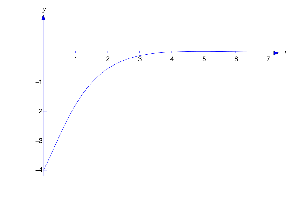
\[ Y(s)={4\over3}{1\over s+1/2}-{8\over s+1}+{8\over3}{1\over s+2}, \]

so the solution of (8.3.14) is

\[ y={\cal L}^{-1}(Y(s))={4\over3}e^{-t/2}-8e^{-t}+{8\over3}e^{-2t} \]

(Figure 8.3.1).

y=43e^-t/2-8e^-t+83e^-2t — Figure 8.3.1. \(y=\dst{{4\over3}e^{-t/2}-8e^{-t}+{8\over3}e^{-2t}}\)

y=12-72e^-tt-52e^-tt — Figure 8.3.2. \(y=\dst{{1\over2}-{7\over2}e^{-t}\cos t-{5\over2}e^{-t}\sin t}\)

Example 8.3.4

Solve the initial value problem

\begin{equation} y''+2y'+2y=1, \quad y(0)=-3,\; y'(0)=1. \tag{8.3.15}\end{equation}

Solution The characteristic polynomial is

\[ p(s)=s^2+2s+2=(s+1)^2+1 \]

and

\[ F(s)={\cal L}(1)={1\over s}, \]

so (8.3.13) becomes

\[ \left[(s+1)^2+1\right] Y(s)={1\over s}+1\cdot(1-3s)+2(-3). \]

Solving for \(Y(s)\) yields

\[ Y(s)={1-s(5+3s)\over s\left[(s+1)^2+1\right]}. \]

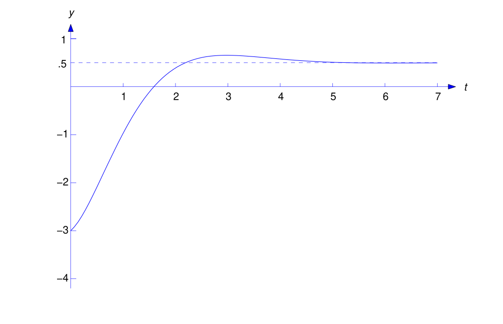
In Example 8.2.8 we found the inverse transform of this function to be

\[ y={1\over2}-{7\over2}e^{-t}\cos t-{5\over2}e^{-t}\sin t \]

(Figure 8.3.2), which is therefore the solution of (8.3.15).

Remark

In our examples we applied Theorems 8.3.1 and 8.3.2 without verifying that the unknown function \(y\) satisfies their hypotheses. This is characteristic of the formal manipulative way in which the Laplace transform is used to solve differential equations. Any doubts about the validity of the method for solving a given equation can be resolved by verifying that the resulting function \(y\) is the solution of the given problem.

8.3 Exercises

In Exercises 1–31 use the Laplace transform to solve the initial value problem.

\(y''+3y'+2y=e^t, \quad y(0)=1,\quad y'(0)=-6\)

Show answer

\(y=\dst{{1\over6}e^t-{9\over 2}e^{-t}+{16\over3}e^{-2t}}\)
\(y''-y'-6y=2, \quad y(0)=1,\quad y'(0)=0\)

Show answer

\(y=\dst{-{1\over3}+{8\over15}e^{3t}+{4\over 5}e^{-2t}}\)
\(y''+y'-2y=2e^{3t}, \quad y(0)=-1,\quad y'(0)=4\)

Show answer

\(y=\dst{-{23\over15}e^{-2t}+{1\over3}e^t +{1\over5}e^{3t}}\)
\(y''-4y=2 e^{3t}, \quad y(0)=1,\quad y'(0)=-1\)

Show answer

\(y=\dst{-{1\over4}e^{2t}+{17\over 20}e^{-2t}+{2\over5}e^{3t}}\)
\(y''+y'-2y=e^{3t}, \quad y(0)=1,\quad y'(0)=-1\)

Show answer

\(y=\dst{{11\over15}e^{-2t}+{1\over 6}e^t+{1\over10}e^{3t}}\)
\(y''+3y'+2y=6e^t, \quad y(0)=1,\quad y'(0)=-1\)

Show answer

\(y=e^t+2e^{-2t}-2e^{-t}\)
\(y''+y=\sin2t, \quad y(0)=0,\quad y'(0)=1\)

Show answer

\(y=\dst{{5\over3}\sin t-{1\over3}\sin2t}\)
\(y''-3y'+2y=2e^{3t}, \quad y(0)=1,\quad y'(0)=-1\)

Show answer

\(y=4e^t-4e^{2t}+e^{3t}\)
\(y''-3y'+2y=e^{4t}, \quad y(0)=1,\quad y'(0)=-2\)

Show answer

\(y=\dst{-{7\over2}e^{2t}+{13\over 3}e^t+{1\over6}e^{4t}}\)
\(y''-3y'+2y=e^{3t}, \quad y(0)=-1,\quad y'(0)=-4\)

Show answer

\(y=\dst{{5\over2}e^t-4e^{2t}+{1\over 2}e^{3t}}\)
\(y''+3y'+2y=2e^t, \quad y(0)=0,\quad y'(0)=-1\)

Show answer

\(y=\dst{{1\over3}e^t-2e^{-t}+{5\over3}e^{-2t}}\)
\(y''+y'-2y=-4, \quad y(0)=2,\quad y'(0)=3\)

Show answer

\(y=2-e^{-2t}+e^t\)
\(y''+4y=4, \quad y(0)=0,\quad y'(0)=1\)

Show answer

\(y=\dst{1-\cos2t+{1\over2}\sin2t}\)
\(y''-y'-6y=2, \quad y(0)=1,\quad y'(0)=0\)

Show answer

\(y=\dst{-{1\over3}+{8\over15}e^{3t} +{4\over5}e^{-2t}}\)
\(y''+3y'+2y=e^t, \quad y(0)=0,\quad y'(0)=1\)

Show answer

\(y=\dst{{1\over6}e^t-{2\over 3}e^{-2t}+{1\over2}e^{-t}}\)
\(y''-y=1, \quad y(0)=1,\quad y'(0)=0\)

Show answer

\(y=-1+e^t+e^{-t}\)
\(y''+4y=3\sin t, \quad y(0)=1,\quad y'(0)=-1\)

Show answer

\(y=\cos2t-\sin2t+\sin t\)
\(y''+y'=2e^{3t}, \quad y(0)=-1,\quad y'(0)=4\)

Show answer

\(y=\dst{{7\over3}-{7\over2}e^{-t} +{1\over6}e^{3t}}\)
\(y''+y=1, \quad y(0)=2,\quad y'(0)=0\)

Show answer

\(y=1+\cos t\)
\(y''+y=t, \quad y(0)=0,\quad y'(0)=2\)

Show answer

\(y=t+\sin t\)
\(y''+y=t-3\sin2t, \quad y(0)=1,\quad y'(0)=-3\)

Show answer

\(y=t-6\sin t+\cos t+\sin2t\)
\(y''+5y'+6y=2e^{-t}, \quad y(0)=1,\quad y'(0)=3\)

Show answer

\(y=e^{-t}+4e^{-2t}-4e^{-3t}\)
\(y''+2y'+y=6\sin t-4\cos t, \quad y(0)=-1,\; y'(0)=1\)

Show answer

\(y=-3\cos t-2\sin t+ e^{-t}(2+5t)\)
\(y''-2y'-3y=10\cos t, \quad y(0)=2,\quad y'(0)=7\)

Show answer

\(y=-\sin t-2\cos t+3e^{3t}+e^{-t}\)
\(y''+y=4\sin t+6\cos t, \quad y(0)=-6,\; y'(0)=2\)

Show answer

\(y=(3t+4)\sin t-(2t+6)\cos t\)
\(y''+4y=8\sin2t+9\cos t, \quad y(0)=1,\quad y'(0)=0\)

Show answer

\(y=-(2t+2)\cos2t+\sin2t+3\cos t\)
\(y''-5y'+6y=10e^t\cos t, \quad y(0)=2,\quad y'(0)=1\)

Show answer

\(y=e^t(\cos t-3\sin t)+e^{3t}\)
\(y''+2y'+2y=2t, \quad y(0)=2,\quad y'(0)=-7\)

Show answer

\(y=-1+t+e^{-t} (3\cos t-5\sin t)\)
\(y''-2y'+2y=5\sin t+10\cos t, \quad y(0)=1,\; y'(0)=2\)

Show answer

\(y=4\cos t-3\sin t-e^{t}(3\cos t-8\sin t)\)
\(y''+4y'+13y=10e^{-t}-36e^t, \quad y(0)=0,\; y'(0)=-16\)

Show answer

\(y=e^{-t}-2e^t+e^{-2t} (\cos 3t-{11/3} \sin3t)\)
\(y''+4y'+5y=e^{-t}(\cos t+3\sin t), \quad y(0)=0,\quad y'(0)=4\)

Show answer

\(y=e^{-t}(\sin t-\cos t)+e^{-2t}(\cos t +4\sin t)\)
\(2y''-3y'-2y=4e^t, \quad y(0)=1,\; y'(0)=-2\)

Show answer

\(y=\dst{{1\over5}e^{2t}-{4\over3}e^t +{32\over15}e^{-t/2}}\)
\(6y''-y'-y=3e^{2t}, \quad y(0)=0,\; y'(0)=0\)

Show answer

\(y=\dst{{1\over7}e^{2t}-{2\over 5}e^{t/2}+{9\over35}e^{-t/3}}\)
\(2y''+2y'+y=2t, \quad y(0)=1,\; y'(0)=-1\)

Show answer

\(y=\dst{e^{-t/2}(5\cos(t/2)-\sin(t/2))+2t-4}\)
\(4y''-4y'+5y=4\sin t-4\cos t, \quad y(0)=0,\; y'(0)=11/17\)

Show answer

\(y=\dst{1\over17}\left(12\cos t+20\sin t-3e^{t/2}(4\cos t+\sin t )\right)\).
\(4y''+4y'+y=3\sin t+\cos t, \quad y(0)=2,\; y'(0)=-1\)

Show answer

\(y=\dst{{e^{-t/2}\over10}(5t+26)-{1\over5}(3\cos t+\sin t)}\)
\(9y''+6y'+y=3e^{3t}, \quad y(0)=0,\; y'(0)=-3\)

Show answer

\(y=\dst{1\over100}\left(3e^{3t}-e^{t/3}(3+310t)\right)\)
Suppose \(a,b\), and \(c\) are constants and \(a\ne0\). Let

\[ y_1={\cal L}^{-1}\left(as+b\over as^2+bs+c\right)\mbox{\quad and \quad} y_2={\cal L}^{-1}\left(a\over as^2+bs+c\right). \]

Show that

\[ y_1(0)=1,\quad y_1'(0)=0\mbox{\quad and \quad} y_2(0)=0,\quad y_2'(0)=1. \]

Hint

Use the Laplace transform to solve the initial value problems

\begin{eqnarray*} ay''+by'+cy&=&0, \quad y(0)=1,\quad y'(0)=0 \\ ay''+by'+cy&=&0, \quad y(0)=0,\quad y'(0)=1. \end{eqnarray*}