The spherical coordinate system is defined with respect to the Cartesian system in Figure 4.16. The spherical system uses \(r\), the distance measured from the origin;[1] \(\theta\), the angle measured from the \(+z\) axis toward the \(z=0\) plane; and \(\phi\), the angle measured in a plane of constant \(z\), identical to \(\phi\) in the cylindrical system.
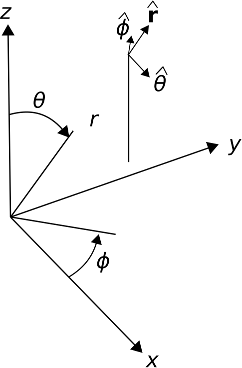
Spherical coordinates are preferred over Cartesian and cylindrical coordinates when the geometry of the problem exhibits spherical symmetry. For example, in the Cartesian coordinate system, the surface of a sphere concentric with the origin requires all three coordinates (\(x\), \(y\), and \(z\)) to describe. However, this surface can be described using a single constant parameter – the radius \(r\) – in the spherical coordinate system. This leads to a dramatic simplification in the mathematics in certain applications.
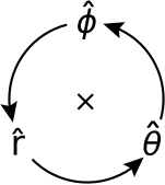
The basis vectors in the spherical system are \(\hat{\bf r}\), \(\hat{\bf \theta}\), and \(\hat{\bf \phi}\). As always, the dot product of like basis vectors is equal to one, and the dot product of unlike basis vectors is equal to zero. For the cross-products, we find:
A useful diagram that summarizes these relationships is shown in Figure 4.17.
Like the cylindrical system, the spherical system is often less useful than the Cartesian system for identifying absolute and relative positions. The reason is the same: Basis directions in the spherical system depend on position. For example, \(\hat{\bf r}\) is directed radially outward from the origin, so \(\hat{\bf r}=\hat{\bf x}\) for locations along the \(x\)-axis but \(\hat{\bf r}=\hat{\bf y}\) for locations along the \(y\) axis and \(\hat{\bf r}=\hat{\bf z}\) for locations along the \(z\) axis. Similarly, the directions of \(\hat{\bf \theta}\) and \(\hat{\bf \phi}\) vary as a function of position. To overcome this awkwardness, it is common to begin a problem in spherical coordinates, and then to convert to Cartesian coordinates at some later point in the analysis. Here are the conversions:
The conversion from Cartesian to spherical coordinates is as follows:
where \(\arctan\) is the four-quadrant inverse tangent function.[2]
Dot products between basis vectors in the spherical and Cartesian systems are summarized in Table 4.2. This information can be used to convert between basis vectors in the spherical and Cartesian systems, in the same manner described in Section 4.3; e.g.
and so on.
| \(\cdot\) | \(\hat{\bf r}\) | \(\hat{\bf \theta}\) | \(\hat{\bf \phi}\) |
| \(\hat{\bf x}\) | \(\sin\theta\cos\phi\) | \(~\cos\theta\cos\phi\) | \(-\sin\phi\) |
| \(\hat{\bf y}\) | \(\sin\theta\sin\phi\) | \(~\cos\theta\sin\phi\) | \(~\cos\phi\) |
| \(\hat{\bf z}\) | \(\cos\theta\) | \(-\sin\theta\) | 0 |
Example 4.3
Cartesian to spherical conversion.
A vector field \({\bf G} = \hat{\bf x}~xz/y\). Develop an expression for \({\bf G}\) in spherical coordinates.
Solution: Simply substitute expressions in terms of spherical coordinates for expressions in terms of Cartesian coordinates. Use Table 4.2 and Equations 4.72–4.74. Making these substitutions and applying a bit of mathematical clean-up afterward, one obtains
Integration Over Length. A differential-length segment of a curve in the spherical system is
Note that \(\theta\) is an angle, as opposed to a distance. The associated distance is \(r~d\theta\) in the \(\theta\) direction. Note also that in the \(\phi\) direction, distance is \(r~d\phi\) in the \(z=0\) plane and less by the factor \(\sin\theta\) for \(z<>0\).
As always, the integral of a vector field \({\bf A}({\bf r})\) over a curve \({\mathcal C}\) is
To demonstrate line integration in the spherical system, imagine a sphere of radius \(a\) centered at the origin with “poles” at \(z=+a\) and \(z=-a\). Let us calculate the integral of \({\bf A}({\bf r})=\hat{\bf \theta}\), where \(\mathcal{C}\) is the arc drawn directly from pole to pole along the surface of the sphere, as shown in Figure 4.18. In this example, \(d{\bf l} = \hat{\bf \theta}~a~d\theta\) since \(r=a\) and \(\phi\) (which could be any value) are both constant along \({\mathcal C}\). Subsequently, \({\bf A}\cdot d{\bf l}=a~d\theta\) and the above integral is
i.e., half the circumference of the sphere, as expected.
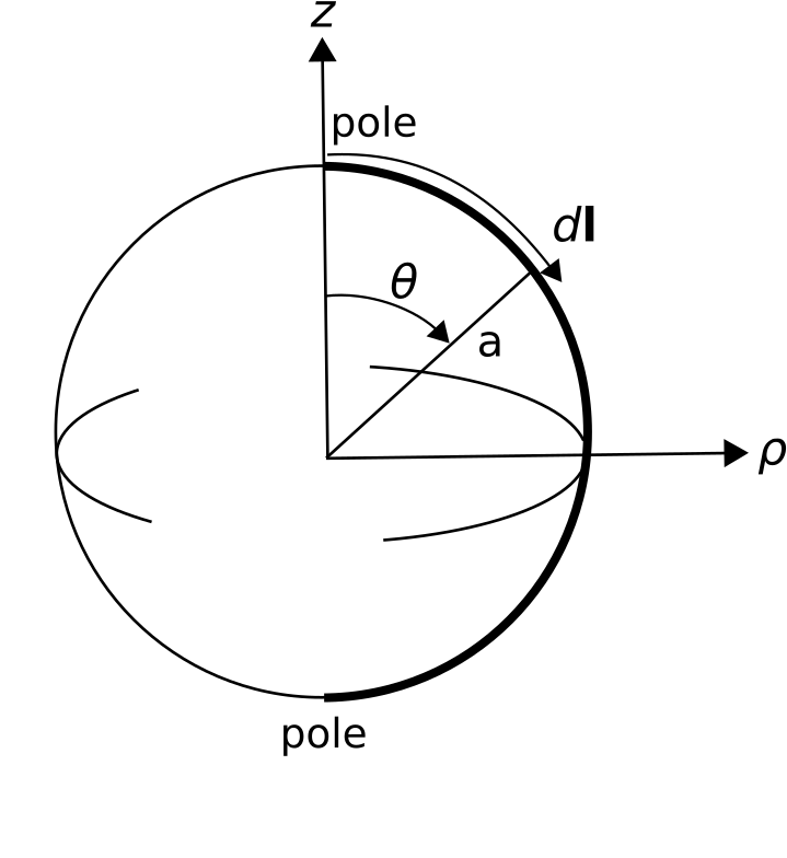
Note that the spherical system is an appropriate choice for this example because the problem can be expressed with the minimum number of varying coordinates in the spherical system. If we had attempted this problem in the Cartesian system, we would find that both \(z\) and either \(x\) or \(y\) (or all three) vary over \({\mathcal C}\) and in a relatively complex way.
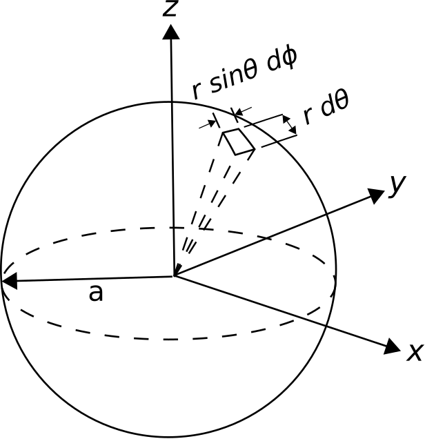
Integration Over Area. Now we ask the question, what is the integral of some vector field \({\bf A}\) over the surface \({\mathcal S}\) of a sphere of radius \(a\) centered on the origin? This is shown in Figure 4.19. The differential surface vector in this case is
As always, the direction is normal to the surface and in the direction associated with positive flux. The quantities in parentheses are the distances associated with varying \(\theta\) and \(\phi\), respectively. In general, the integral over a surface is
In this case, let’s consider \({\bf A}=\hat{\bf r}\); in this case \({\bf A}\cdot d{\bf s} = a^2~\sin\theta~d\theta~d\phi\) and the integral becomes
which we recognize as the area of the sphere, as expected. The corresponding calculation in the Cartesian or cylindrical systems is quite difficult in comparison.
Integration Over Volume. The differential volume element in the spherical system is
For example, if \(A({\bf r})=1\) and the volume \(\mathcal{V}\) is a sphere of radius \(a\) centered on the origin, then
which is the volume of a sphere.
Additional Reading:
“Spherical coordinate system” on Wikipedia.