Cartesian coordinates (Section 4.2) are not convenient in certain cases. One of these is when the problem has cylindrical symmetry. For example, in the Cartesian coordinate system, the cross-section of a cylinder concentric with the \(z\)-axis requires two coordinates to describe: \(x\) and \(y\). However, this cross section can be described using a single parameter – namely the radius – which is \(\rho\) in the cylindrical coordinate system. This results in a dramatic simplification of the mathematics in some applications.
The cylindrical system is defined with respect to the Cartesian system in Figure 4.11. In lieu of \(x\) and \(y\), the cylindrical system uses \(\rho\), the distance measured from the closest point on the \(z\) axis,[1] and \(\phi\), the angle measured in a plane of constant \(z\), beginning at the \(+x\) axis (\(\phi=0\)) with \(\phi\) increasing toward the \(+y\) direction.
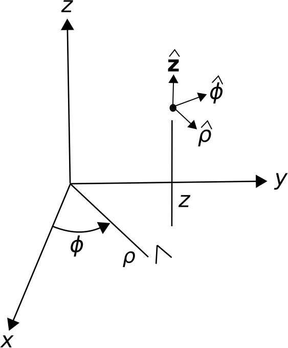
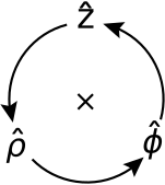
The basis vectors in the cylindrical system are \(\hat{\bf \rho}\), \(\hat{\bf \phi}\), and \(\hat{\bf z}\). As in the Cartesian system, the dot product of like basis vectors is equal to one, and the dot product of unlike basis vectors is equal to zero. The cross products of basis vectors are as follows:
A useful diagram that summarizes these relationships is shown in Figure 4.12.
The cylindrical system is usually less useful than the Cartesian system for identifying absolute and relative positions. This is because the basis directions depend on position. For example, \(\hat{\bf \rho}\) is directed radially outward from the \(\hat{\bf z}\) axis, so \(\hat{\bf \rho}=\hat{\bf x}\) for locations along the \(x\)-axis but \(\hat{\bf \rho}=\hat{\bf y}\) for locations along the \(y\) axis. Similarly, the direction \(\hat{\bf \phi}\) varies as a function of position. To overcome this awkwardness, it is common to set up a problem in cylindrical coordinates in order to exploit cylindrical symmetry, but at some point to convert to Cartesian coordinates. Here are the conversions:
and \(z\) is identical in both systems. The conversion from Cartesian to cylindrical is as follows:
where \(\arctan\) is the four-quadrant inverse tangent function; i.e., \(\arctan(y/x)\) in the first quadrant (\(x>0\), \(y>0\)), but possibly requiring an adjustment for the other quadrants because the signs of both \(x\) and \(y\) are individually significant.[2]
Similarly, it is often necessary to represent basis vectors of the cylindrical system in terms of Cartesian basis vectors and vice-versa. Conversion of basis vectors is straightforward using dot products to determine the components of the basis vectors in the new system. For example, \(\hat{\bf x}\) in terms of the basis vectors of the cylindrical system is
The last term is of course zero since \(\hat{\bf z}\cdot\hat{\bf x}=0\). Calculation of the remaining terms requires dot products between basis vectors in the two systems, which are summarized in Table 4.1. Using this table, we find
and of course \(\hat{\bf z}\) requires no conversion. Going from Cartesian to cylindrical, we find
| \(\cdot\) | \(\hat{\bf \rho}\) | \(\hat{\bf \phi}\) | \(\hat{\bf z}\) |
| \(\hat{\bf x}\) | \(\cos\phi\) | \(-\sin\phi\) | 0 |
| \(\hat{\bf y}\) | \(\sin\phi\) | \(~\cos\phi\) | 0 |
| \(\hat{\bf z}\) | 0 | 0 | 1 |
Integration Over Length. A differential-length segment of a curve in the cylindrical system is described in general as
Note that the contribution of the \(\phi\) coordinate to differential length is \(\rho d\phi\), not simply \(d\phi\). This is because \(\phi\) is an angle, not a distance. To see why the associated distance is \(\rho d\phi\), consider the following. The circumference of a circle of radius \(\rho\) is \(2\pi\rho\). If only a fraction of the circumference is traversed, the associated arclength is the circumference scaled by \(\phi/2\pi\), where \(\phi\) is the angle formed by the traversed circumference. Therefore, the distance is \(2\pi\rho \cdot \phi/2\pi = \rho \phi\), and the differential distance is \(\rho d\phi\).
As always, the integral of a vector field \({\bf A}({\bf r})\) over a curve \({\mathcal C}\) is
To demonstrate the cylindrical system, let us calculate the integral of \({\bf A}({\bf r})=\hat{\bf \phi}\) when \(\mathcal{C}\) is a circle of radius \(\rho_0\) in the \(z=0\) plane, as shown in Figure 4.13. In this example, \(d{\bf l} = \hat{\bf \phi}~\rho_0~d\phi\) since \(\rho=\rho_0\) and \(z=0\) are both constant along \({\mathcal C}\). Subsequently, \({\bf A}\cdot d{\bf l}=\rho_0 d\phi\) and the above integral is
i.e., this is a calculation of circumference.
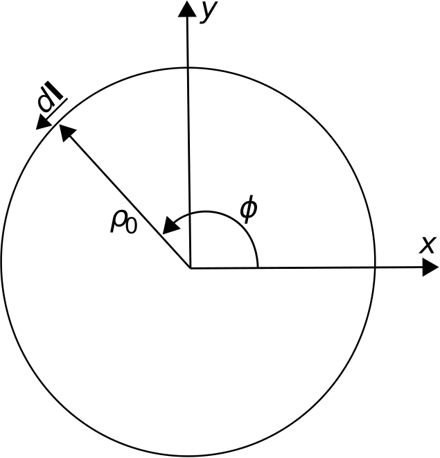
Note that the cylindrical system is an appropriate choice for the preceding example because the problem can be expressed with the minimum number of varying coordinates in the cylindrical system. If we had attempted this problem in the Cartesian system, we would find that both \(x\) and \(y\) vary over \({\mathcal C}\), and in a relatively complex way.[3]
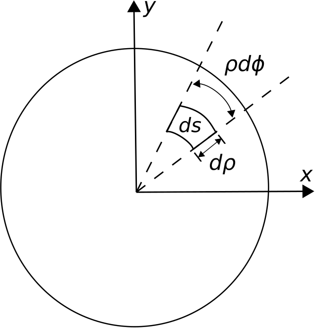
Integration Over Area. Now we ask the question, what is the integral of some vector field \({\bf A}\) over a circular surface \({\mathcal S}\) in the \(z=0\) plane having radius \(\rho_0\)? This is shown in Figure 4.14. The differential surface vector in this case is
The quantities in parentheses are the radial and angular dimensions, respectively. The direction of \(d{\bf s}\) indicates the direction of positive flux – see the discussion in Section 4.2 for an explanation. In general, the integral over a surface is
To demonstrate, let’s consider \({\bf A}=\hat{\bf z}\); in this case \({\bf A}\cdot d{\bf s} = \rho~d\rho~d\phi\) and the integral becomes
which we recognize as the area of the circle, as expected. The corresponding calculation in the Cartesian system is quite difficult in comparison.
Whereas the previous example considered a planar surface, we might consider instead a curved surface. Here we go. What is the integral of a vector field \({\bf A}=\hat{\bf \rho}\) over a cylindrical surface \({\mathcal S}\) concentric with the \(z\) axis having radius \(\rho_0\) and extending from \(z=z_1\) to \(z=z_2\)? This is shown in Figure 4.15.
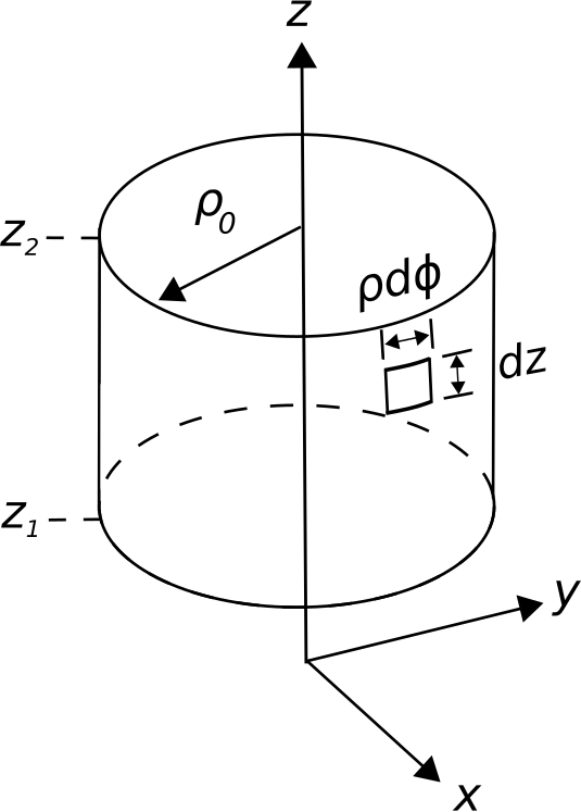
The differential surface vector in this case is
The integral is
which is the area of \({\mathcal S}\), as expected. Once again, the corresponding calculation in the Cartesian system is quite difficult in comparison.
Integration Over Volume. The differential volume element in the cylindrical system is
For example, if \(A({\bf r})=1\) and the volume \(\mathcal{V}\) is a cylinder bounded by \(\rho\le \rho_0\) and \(z_1\le z \le z_2\), then
i.e., area times length, which is volume.
Once again, the procedure above is clearly more complicated than is necessary if we are interested only in computing volume. However, if the integrand is not constant-valued then we are no longer simply computing volume. In this case, the formalism is appropriate and possibly necessary.
Additional Reading:
“Cylindrical coordinate system” on Wikipedia.