Let us now consider the input impedance of a transmission line that is terminated in an open- or short-circuit. Such a transmission line is sometimes referred to as a stub. First, why consider such a thing? From a “lumped element” circuit theory perspective, this would not seem to have any particular application. However, the fact that this structure exhibits an input impedance that depends on length (Section 3.15) enables some very useful applications.
First, let us consider the question at hand: What is the input impedance when the transmission line is open- or short-circuited? For a short circuit, \(Z_L=0\), \(\Gamma=-1\), so we find
Multiplying numerator and denominator by \(e^{+j\beta l}\) we obtain
Now we invoke the following trigonometric identities:
Employing these identities, we obtain:
and finally:
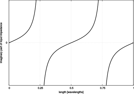
Figure 3.23(a) shows what’s going on. As expected, \(Z_{in}=0\) when \(l=0\), since this amounts to a short circuit with no transmission line. Also, \(Z_{in}\) varies periodically with increasing length, with period \(\lambda/2\). This is precisely as expected from standing wave theory (Section 3.13). What is of particular interest now is that as \(l\rightarrow\lambda/4\), we see \(Z_{in}\rightarrow\infty\). Remarkably, the transmission line has essentially transformed the short circuit termination into an open circuit!
For an open circuit termination, \(Z_L\rightarrow\infty\), \(\Gamma=+1\), and we find
Following the same procedure detailed above for the short-circuit case, we find
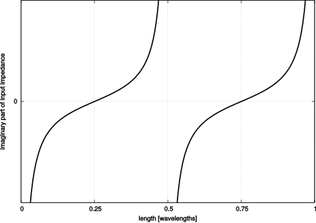
Figure 3.23(b) shows the result for open-circuit termination. As expected, \(Z_{in}\rightarrow\infty\) for \(l=0\), and the same \(\lambda/2\) periodicity is observed. What is of particular interest now is that at \(l=\lambda/4\) we see \(Z_{in}=0\). In this case, the transmission line has transformed the open circuit termination into a short circuit.
Now taking stock of what we have determined:
The input impedance of a short- or open-circuited lossless transmission line is completely imaginary-valued and is given by Equations 3.117 and 3.119, respectively.
The input impedance of a short- or open-circuited lossless transmission line alternates between open- (\(Z_{in}\rightarrow\infty\)) and short-circuit (\(Z_{in}=0\)) conditions with each \(\lambda/4\)-increase in length.
Additional Reading:
“Stub (electronics)” on Wikipedia.