Consider Figure 3.22, which shows a lossless transmission line being driven from the left and which is terminated by an impedance \(Z_L\) on the right. If \(Z_L\) is equal to the characteristic impedance \(Z_0\) of the transmission line, then the input impedance \(Z_{in}\) will be equal to \(Z_L\). Otherwise \(Z_{in}\) depends on both \(Z_L\) and the characteristics of the transmission line. In this section, we determine a general expression for \(Z_{in}\) in terms of \(Z_L\), \(Z_0\), the phase propagation constant \(\beta\), and the length \(l\) of the line.
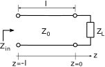
Using the coordinate system indicated in Figure 3.22, the interface between source and transmission line is located at \(z=-l\). Impedance is defined at the ratio of potential to current, so:
Now employing expressions for \(\widetilde{V}(z)\) and \(\widetilde{I}(z)\) from Section 3.13 with \(z=-l\), we find:
Multiplying both numerator and denominator by \(e^{-j\beta l}\):
Recall that \(\Gamma\) in the above expression is:
Summarizing:
Equation 3.109 is the input impedance of a lossless transmission line having characteristic impedance \(Z_0\) and which is terminated into a load \(Z_L\). The result also depends on the length and phase propagation constant of the line.
Note that \(Z_{in}(l)\) is periodic in \(l\). Since the argument of the complex exponential factors is \(2\beta l\), the frequency at which \(Z_{in}(l)\) varies is \(\beta/\pi\); and since \(\beta=2\pi/\lambda\), the associated period is \(\lambda/2\). This is very useful to keep in mind because it means that all possible values of \(Z_{in}(l)\) are achieved by varying \(l\) over \(\lambda/2\). In other words, changing \(l\) by more than \(\lambda/2\) results in an impedance which could have been obtained by a smaller change in \(l\). Summarizing to underscore this important idea:
The input impedance of a terminated lossless transmission line is periodic in the length of the transmission line, with period \(\lambda/2\).
Not surprisingly, \(\lambda/2\) is also the period of the standing wave (Section 3.13). This is because – once again – the variation with length is due to the interference of incident and reflected waves.
Also worth noting is that Equation 3.109 can be written entirely in terms of \(Z_L\) and \(Z_0\), since \(\Gamma\) depends only on these two parameters. Here’s that version of the expression:
This expression can be derived by substituting Equation 3.110 into Equation 3.109 and is left as an exercise for the student.
Finally, note that the argument \(\beta l\) appearing Equations 3.109 and 3.111 has units of radians and is referred to as electrical length. Electrical length can be interpreted as physical length expressed with respect to wavelength and has the advantage that analysis can be made independent of frequency.