2.5 Stationary value of an integral

In analytic mechanics, we will find that we need to find the stationary value of an integral. For example, we may need to find the curve \(y(x)\) that results in the definite integral of some function \(L(y,y',x)\) being maximized (or stationary). We called the definite integral, \(I\), a “functional”:

\begin{align} I = \int_a^b L(y,y',x)dx \tag{2.37}\end{align}

One common example is the “Brachistochrone” problem, in which we wish to find the shape of a wire, \(y(x)\), that minimizes the time for a frictionless bead to slide down under gravity from some point \(a\) to another point \(b\). This problem in fact led to the development of the field of variational calculus.

Example 2-4

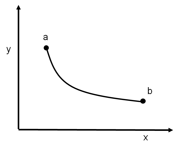
Derive the functional corresponding to a bead sliding under gravity down a frictionless wire given by the function \(y(x)\)

bchrone — Figure 2.2Bead sliding under gravity on a wire from a to b.

The time that it takes to slide down the path is given by the integral of the time it takes to slide down an infinitesimal arc, \(ds\):

\begin{align*} T=\int_a^b \frac{ds}{v} \end{align*}

where v is the instantaneous speed. The speed is easily found by conservation of energy. If the bead started at rest:

\begin{align*} \frac{1}{2}mv^2=mg(y_a-y)\nonumber\\ \therefore v =\sqrt{2g(y_a-y)} \end{align*}

The arc-length, \(ds\), can be expressed in terms of \(dx\) and \(dy\):

\begin{align*} ds=\sqrt{dx^2+dy^2}=\sqrt{1+y'^2}dx \end{align*}

Finally, the time is given by:

\begin{align*} T=\int_a^b \frac{\sqrt{1+y'^2}}{\sqrt{2g(y_a-y)}}dx \end{align*}

And the problem is that of solving for the function \(y(x)\) that minimizes the “functional” \(T\), given by the definite integral of \(L(y,y',x)\), where:

\begin{align*} L(y,y',x)=\frac{\sqrt{1+y'^2}}{\sqrt{2g(y_a-y)}} \end{align*}

We thus want to find the condition on \(L\) such that the functional, \(I\), is stationary, given the boundary condition that the function, \(y(x)\), passes through \(a\) and \(b\).

In analogy with finding the stationary point of a function, we examine the rate of change of the functional as we vary \(y(x)\). We start with the variation of the integrand:

\begin{align} \delta L(y,y',x)=L(y+\delta y, y'+\delta y', x)-L(y,y',x) \tag{2.38}\end{align}

where, as you recall, we do not consider any variations in \(x\). We can use the first order terms in \(\delta\) from a Taylor series to expand \(L(y+\delta y, y'+\delta y', x)\):

\begin{align} L(y+\delta y, y'+\delta y', x)=L(y,y',x)+\frac{\partial L}{\partial y}\delta y+\frac{\partial L}{\partial y'}\delta y' \tag{2.39}\end{align}

Thus:

\begin{align} \delta I &= \delta \int_a^b L(y,y',x)dx\\ &= \int_a^b \delta L(y,y',x)dx\\ &= \int_a^b \left( \frac{\partial L}{\partial y}\delta y+\frac{\partial L}{\partial y'}\delta y'\right)dx \tag{2.40}\end{align}

Recalling from equations 2.2 and 2.6 that we can write:

\begin{align} \delta y = \epsilon \phi(x)\\ \delta y' = \epsilon \phi'(x) \tag{2.41}\end{align}

where \(\phi(x)\) is a small variation of the function \(y(x)\). The functional becomes:

\begin{align} \delta I &=\epsilon \int_a^b \left( \frac{\partial L}{\partial y}\phi(x)+\frac{\partial L}{\partial y'}\phi'(x)\right)dx \tag{2.42}\end{align}

Now, since we want to find a stationary value of \(I\), we require the rate of change of \(\delta I\) with respect to \(\epsilon\) to be zero:

\begin{align} \frac{d\delta I}{d\epsilon}=\frac{\delta I}{\epsilon} &=\int_a^b \left( \frac{\partial L}{\partial y}\phi(x)+\frac{\partial L}{\partial y'}\phi'(x)\right)dx=0 \tag{2.43}\end{align}

The second part can be integrated by parts:

\begin{align} \int_a^b \frac{\partial L}{\partial y'}\phi'(x)dx=\phi(x)\frac{\partial L}{\partial y'}\Big |_a^b-\int_a^b \frac{d}{dx}\left(\frac{\partial L}{\partial y'}\right)\phi(x)dx \tag{2.44}\end{align}

The first term of integration by parts is zero, because the function \(y(x)\) is fixed at the end points of the integration range, so \(\phi(x=a)=\phi(x=b)=0\). We thus have:

\begin{align} \frac{\delta I}{\epsilon} &=\int_a^b \left( \frac{\partial L}{\partial y}\phi(x)-\frac{d}{dx}\left(\frac{\partial L}{\partial y'}\right)\phi(x)\right)dx\\ &=\int_a^b \phi(x)\left( \frac{\partial L}{\partial y}-\frac{d}{dx}\left(\frac{\partial L}{\partial y'}\right)\right)dx=0 \tag{2.45}\end{align}

The only way for this integral to vanish, regardless of the choice of \(\phi(x)\) is for the remaining part of the integrand to always be zero. This leads to the “Euler-Lagrange” equation, which is the condition for the functional \(\int L(y,y',x)dx\) to be stationary:

\begin{align} \frac{d}{dx}\left(\frac{\partial L}{\partial y'}\right)-\frac{\partial L}{\partial y}=0 \tag{2.46}\end{align}

Noting that \(\phi(x)=\delta y\), we could also have written equation 2.45 as:

\begin{align} \frac{\delta I}{\epsilon} &=\int_a^b \delta y\left( \frac{\partial L}{\partial y}-\frac{d}{dx}\left(\frac{\partial L}{\partial y'}\right)\right)dx=0 \tag{2.47}\end{align}

a notation which we will find convenient in the next section.

In analytic mechanics, we will generally have a function, \(L\), that depends on multiple coordinates, \(q_i\), their generalized velocities, \(\dot{q}\), and time will play the role of the independent variable:

\begin{align} L=L(q_1,q_2,\dots,\dot{q_1}, \dot{q_2},\dots,t) \tag{2.48}\end{align}

We will want to find the values of \(q_i(t)\) that lead to a stationary value of:

\begin{align} S=\int_a^b L(q_1,q_2,\dots,\dot{q_1}, \dot{q_2},\dots,t)dt \tag{2.49}\end{align}

Following the same procedure as above, and collecting the terms for each coordinate, we can show that we get an Euler-Lagrange equation for each coordinate:

\begin{align} \frac{d}{dt}\left(\frac{\partial L}{\partial \dot{q}_i}\right)-\frac{\partial L}{\partial q_i}=0 \text{ (i=1…n)} \tag{2.50}\end{align}