where \(\epsilon\) is a number that we can make arbitrarily small, and \(\phi(x)\) is a function that is continuous and differentiable in some interval \(x=a\dots b\) over which \(f(x)\) is defined, continuous and differentiable. We define the variation of a function as:
\begin{align}
\delta y \equiv \bar{f}(x) -f(x) = \epsilon \phi(x)
\tag{2.2}\end{align}
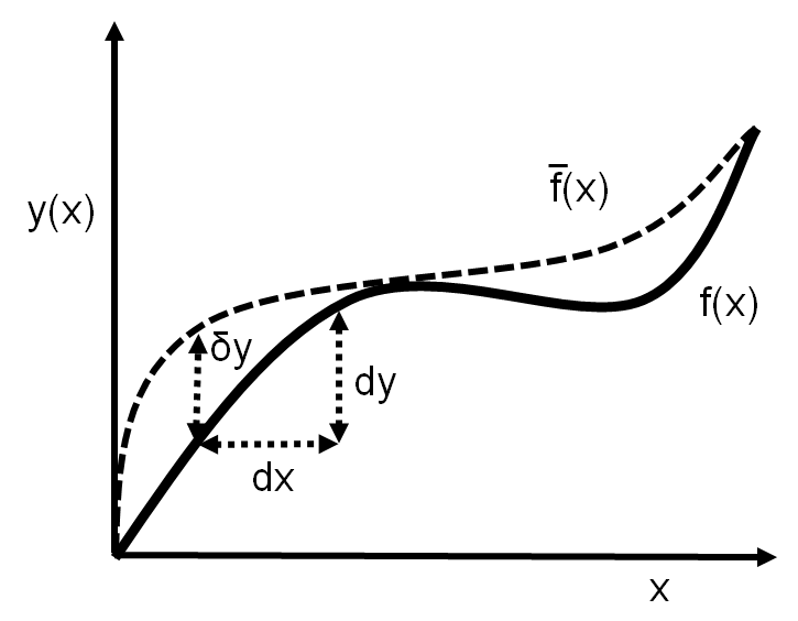
The change in \(f(x)\) is infinitesimal and “virtual”, meaning that we can choose any arbitrary well behaved \(\phi(x)\). Thus \(\delta y\) does not represent a “real” change in the function from a change in its dependent variables. Again, note the difference between \(\delta y\) and \(dy\); \(dy\) is the (familiar) change in \(f(x)\) from a corresponding change in \(x\) by \(dx\), while \(\delta y\) is a change in \(f(x)\) without a change in \(x\), and is a new function. This is illustrated in Figure 2.1.
Figure 2.1A function \(y=f(x)\) showing a differential change \(dx\) which corresponds to a change in \(x\) of \(dx\). The variation of the function at a point, \(\delta y\), is also shown, which is independent of a change in \(x\) and leads to a different function, \(\bar{f}(x)\).
For the calculus of variations, we only consider changes in the dependent variables, thus:
\begin{align}
\delta x = 0
\tag{2.3}\end{align}
Properties of the \(\delta\) operator
Commutation with differentiation
Consider the “derivative of the variation”:
\begin{align}
\frac{d}{dx}\delta y =\frac{d}{dx} \left[\bar{f}(x)-f(x) \right]=\frac{d}{dx} \epsilon \phi(x)=\epsilon \phi'(x)
\tag{2.4}\end{align}
where we have used an apostrophe (’) to designate derivatives with respect to \(x\). Now consider the “variation of the derivative”:
If the function \(F\) is a function of multiple functions, \(y(x), z(x), \dots\), we proceed the same way, but using partial derivatives:
\begin{align}
\delta F(y,z,\dots) &= F(y+\delta y, z+\delta z, \dots)-F(y,z,\dots)\\
&=\frac{\partial F}{\partial y}\delta y +\frac{\partial F}{\partial z}\delta z+\dots+ \frac{1}{2!}\left(\frac{\partial^2F}{\partial y}\delta^2y+\frac{\partial^2F}{\partial z}\delta^2z+2\frac{\partial^2 F}{\partial y\partial z}\delta y \delta z+\dots \right) +\dots
\tag{2.11}\end{align}
where again, we will neglect the terms in \(\delta^2\) and higher.
Example 2-2
Compare the differential displacement and virtual displacement of a position vector \(\vec{r}=\vec{r}(q_1,q_2,\dots,q_n,t)\) that is a function of generalized coordinates, \(q\).
When considering the position of a particle as a function of the generalized coordinates: