1.8 Vector-Valued Functions

Now that we are familiar with vectors and their operations, we can begin discussing functions whose values are vectors.

Definition 1.10

A vector-valued function of a real variable is a rule that associates a vector $\textbf{f}(t)$ with a real number $t$, where $t$ is in some subset $D$ of $\Real{1}$ (called the domain of f). We write $\textbf{f}: D \rightarrow \Real{3}$ to denote that f is a mapping of $D$ into $\Real{3}$.

For example, $\textbf{f}(t) = t \textbf{i} + t^2 \textbf{j} + t^3 \textbf{k}$ is a vector-valued function in $\Real{3}$, defined for all real numbers $t$. We would write $\textbf{f}: \mathbb{R} \rightarrow \Real{3}$. At $t = 1$ the value of the function is the vector $\textbf{i} + \textbf{j} + \textbf{k}$, which in Cartesian coordinates has the terminal point $(1,1,1)$.

A vector-valued function of a real variable can be written in component form as

\[\textbf{f}(t) = \ssub{f}{1}(t) \textbf{i} + \ssub{f}{2}(t) \textbf{j} + \ssub{f}{3}(t) \textbf{k}\]

or in the form

\[\textbf{f}(t) = ( \ssub{f}{1}(t),\ssub{f}{2}(t),\ssub{f}{3}(t) )\]

for some real-valued functions $\ssub{f}{1}(t)$, $\ssub{f}{2}(t)$, $\ssub{f}{3}(t)$, called the component functions of f. The first form is often used when emphasizing that $\textbf{f}(t)$ is a vector, and the second form is useful when considering just the terminal points of the vectors. By identifying vectors with their terminal points, a curve in space can be written as a vector-valued function.

width height 0.5pt

tikzpicture arrows snakes spherecolorHTML80DCFF planecolorHTMLFFB270 [rotate=-90][snake=coil,segment amplitude=1.1cm,segment length=.8cm,segment aspect=0.4] (-1.4,0) -- (1.5,0); [black!60,line width=0.3pt,-latex] (0,0) -- (2,0,0); [black!60,line width=0.3pt,-latex] (0,-1.5) -- (0,2,0); [black!60,line width=0.3pt,-latex] (0,0) -- (0,0,4); 1.90.20 [center,center]y; 0.21.90 [center,center]z; 0.203.8 [center,center]x; 0.05-0.20 [center,center]0; (0,0,1.75) circle (1.5pt); [below,left] at (-0.1,-0.1,1.78) f(0); (0,0.8,1.75) circle (1.5pt); [below,left] at (0,0.64,1.75) f(2 ); tikzpicture

Example 1.35

Define $\textbf{f}: \mathbb{R} \rightarrow \Real{3}$ by $\textbf{f}(t) = ( \cos t , \sin t , t )$.
This is the equation of a helix (see Figure 1.8.1). As the value of $t$ increases, the terminal points of $\textbf{f}(t)$ trace out a curve spiraling upward. For each $t$, the $x$- and $y$-coordinates of $\textbf{f}(t)$ are $x = \cos t$ and $y = \sin t$, so

\[x^2 + y^2 = \cos^2 t + \sin^2 t = 1.\]

Thus, the curve lies on the surface of the right circular cylinder $x^2 + y^2 = 1$.

width height 0.5pt

It may help to think of vector-valued functions of a real variable in $\Real{3}$ as a generalization of the parametric functions in $\Real{2}$ which you learned about in single-variable calculus. Much of the theory of real-valued functions of a single real variable can be applied to vector-valued functions of a real variable. Since each of the three component functions are real-valued, it will sometimes be the case that results from single-variable calculus can simply be applied to each of the component functions to yield a similar result for the vector-valued function. However, there are times when such generalizations do not hold (see Exercise 13). The concept of a limit, though, can be extended naturally to vector-valued functions, as in the following definition.

Definition 1.11

Let $\textbf{f}(t)$ be a vector-valued function, let $a$ be a real number and let c be a vector. Then we say that the limit of $\textbf{f}(t)$ as $t$ approaches $a$ equals c, written as $\lim\limits_{t \to a} \textbf{f}(t) = \textbf{c}$, if $\lim\limits_{t \to a} \,\norm{\textbf{f}(t) - \textbf{c}} = 0$. If $\textbf{f}(t) = ( \ssub{f}{1}(t),\ssub{f}{2}(t),\ssub{f}{3}(t) )$, then

\[\lim_{t \to a} \textbf{f}(t) = \biggl( \lim_{t \to a} \ssub{f}{1}(t), \lim_{t \to a} \ssub{f}{2}(t), \lim_{t \to a} \ssub{f}{3}(t) \biggr)\]

provided that all three limits on the right side exist.

The above definition shows that continuity and the derivative of vector-valued functions can also be defined in terms of its component functions.

Definition 1.12

Let $\textbf{f}(t) = ( \ssub{f}{1}(t),\ssub{f}{2}(t),\ssub{f}{3}(t) )$ be a vector-valued function, and let $a$ be a real number in its domain. Then $\textbf{f}(t)$ is continuous at $a$ if $\lim\limits_{t \to a} \textbf{f}(t) = \textbf{f}(a)$. Equivalently, $\textbf{f}(t)$ is continuous at $a$ if and only if $\ssub{f}{1}(t)$, $\ssub{f}{2}(t)$, and $\ssub{f}{3}(t)$ are continuous at $a$.
The derivative of $\textbf{f}(t)$ at $a$, denoted by $\textbf{f}\,'(a)$ or $\dfrac{d \textbf{f}}{dt}(a)$, is the limit

\[\textbf{f}\,'(a) = \lim_{h \to 0} \frac{\textbf{f}(a + h) - \textbf{f}(a)}{h}\]

if that limit exists. Equivalently, $\textbf{f}\,'(a) = ( \ssub{f}{1}\,'(a),\ssub{f}{2}\,'(a), \ssub{f}{3}\,'(a) )$, if the component derivatives exist. We say that $\textbf{f}(t)$ is differentiable at $a$ if $\textbf{f}\,'(a)$ exists.

Recall that the derivative of a real-valued function of a single variable is a real number, representing the slope of the tangent line to the graph of the function at a point. Similarly, the derivative of a vector-valued function is a tangent vector to the curve in space which the function represents, and it lies on the tangent line to the curve (see Figure 1.8.1).

tikzpicture arrows [black!60,line width=0.3pt,-latex] (0,0) -- (6,0,0); [black!60,line width=0.3pt,-latex] (0,0) -- (0,2.8,0); [black!60,line width=0.3pt,-latex] (0,0) -- (0,0,2); 5.90.20 [center,center]y; 0.22.70 [center,center]z; 0.201.8 [center,center]x; 0.05-0.20 [center,center]0; [blue!60,line width=0.3pt] (1.2,2.51) -- (5.2,1.79); [rounded corners,line width=0.6pt](0.75,2.1) .. controls (2.95,3) and (3.55,1.2) .. (4,0.75) .. controls (4.3,0.45) and (4.9,0.3) .. (5.35,0.6); [black,line width=1.2pt,-latex] (0,0) -- (2.2,2.3); [black,line width=1.2pt,-latex] (0,0) -- (4.22,0.55); [black,line width=1.2pt,-latex] (2.2,2.3) -- (4.22,0.55); [black,line width=1.2pt,-latex] (2.2,2.33) -- (3.7,2.06); [above] at (5.2,1.79) L; [above] at (5.35,0.6) f(t); [above] at (3.7,2.06) f\,'(a); [left,above] at (1,1.2) f(a); [below] at (3.8,0.5) f(a + h); [below,rotate=-40] at (3.05,1.52) f(a + h) - f(a); tikzpicture — Figure 1.8.1Tangent vector $\textbf{f}\,'(a)$ and tangent line $L = \textbf{f}(a) + s \textbf{f}\,'(a)$

width height 0.5pt

Example 1.36

Let $\textbf{f}(t) = ( \cos t , \sin t , t )$. Then $\textbf{f}\,'(t) = ( -\sin t , \cos t , 1 )$ for all $t$. The tangent line $L$ to the curve at $\textbf{f}(2\pi) = (1,0,2\pi)$ is $L = \textbf{f}(2\pi) + s\,\textbf{f}\,'(2\pi) = (1,0,2\pi) + s(0,1,1)$, or in parametric form: $x = 1$, $y = s$, $z = 2\pi + s$ for $-\infty < s < \infty$.

width height 0.5pt A scalar function is a real-valued function. Note that if $u(t)$ is a scalar function and $\textbf{f}(t)$ is a vector-valued function, then their product, defined by $(u\,\textbf{f})(t) = u(t)\,\textbf{f}(t)$ for all $t$, is a vector-valued function (since the product of a scalar with a vector is a vector).

The basic properties of derivatives of vector-valued functions are summarized in the following theorem.

Theorem 1.20

Let $\textbf{f}(t)$ and $\textbf{g}(t)$ be differentiable vector-valued functions, let $u(t)$ be a differentiable scalar function, let $k$ be a scalar, and let c be a constant vector. Then

(a) $\dfrac{d}{dt} ( \textbf{c} ) = \textbf{0}$

(b) $\dfrac{d}{dt} ( k \textbf{f} ) = k \dfrac{d \textbf{f}}{dt}$

(d) $\dfrac{d}{dt} ( \textbf{f} - \textbf{g} ) = \dfrac{d \textbf{f}}{dt} \,-\, \dfrac{d \textbf{g}}{dt}$

(e) $\dfrac{d}{dt} ( u\,\textbf{f} ) = \dfrac{du}{dt}\,\textbf{f} \,+\, u \dfrac{d \textbf{f}}{dt}$

(f) $\dfrac{d}{dt} ( \Dotprod{\textbf{f}}{\textbf{g}} ) = \Dotprod{\dfrac{d \textbf{f}}{dt}}{\textbf{g}} \,+\, \Dotprod{\textbf{f}}{\dfrac{d \textbf{g}}{dt}}$

(g) $\dfrac{d}{dt} ( \Crossprod{\textbf{f}\,}{\,\textbf{g}} ) = \Crossprod{\dfrac{d \textbf{f}}{dt}}{\,\textbf{g}} \,+\, \Crossprod{\textbf{f}\,}{\dfrac{d \textbf{g}}{dt}}$

proof[Proof:] The proofs of parts (a)-(e) follow easily by differentiating the component functions and using the rules for derivatives from single-variable calculus. We will prove part (f), and leave the proof of part (g) as an exercise for the reader.
(f) Write $\textbf{f}(t) = ( \ssub{f}{1}(t),\ssub{f}{2}(t),\ssub{f}{3}(t) )$ and $\textbf{g}(t) = ( \ssub{g}{1}(t),\ssub{g}{2}(t),\ssub{g}{3}(t) )$, where the component functions $\ssub{f}{1}(t)$, $\ssub{f}{2}(t)$, $\ssub{f}{3}(t)$, $\ssub{g}{1}(t)$, $\ssub{g}{2}(t)$, $\ssub{g}{3}(t)$ are all differentiable real-valued functions. Then

\begin{align*}\begin{split} \dfrac{d}{dt} ( \Dotprod{\textbf{f}(t)}{\textbf{g}(t)} ) &= \dfrac{d}{dt} ( \ssub{f}{1}(t)\,\ssub{g}{1}(t) + \ssub{f}{2}(t)\,\ssub{g}{2}(t) + \ssub{f}{3}(t)\,\ssub{g}{3}(t) )\\ &= \dfrac{d}{dt} ( \ssub{f}{1}(t)\,\ssub{g}{1}(t) ) + \dfrac{d}{dt} ( \ssub{f}{2}(t)\,\ssub{g}{2}(t) ) + \dfrac{d}{dt} ( \ssub{f}{3}(t)\,\ssub{g}{3}(t) )\\ &= \dfrac{d\ssub{f}{1}}{dt}(t)\,\ssub{g}{1}(t) + \ssub{f}{1}(t)\,\dfrac{d\ssub{g}{1}}{dt}(t) + \dfrac{d\ssub{f}{2}}{dt}(t)\,\ssub{g}{2}(t) + \ssub{f}{2}(t)\,\dfrac{d\ssub{g}{2}}{dt}(t) + \dfrac{d\ssub{f}{3}}{dt}(t)\,\ssub{g}{3}(t) + \ssub{f}{3}(t)\,\dfrac{d\ssub{g}{3}}{dt}(t)\\ &= \Dotprod{\biggl( \dfrac{d\ssub{f}{1}}{dt}(t),\dfrac{d\ssub{f}{2}}{dt}(t),\dfrac{d\ssub{f}{3}}{dt}(t) \biggr)}{ ( \ssub{g}{1}(t),\ssub{g}{2}(t),\ssub{g}{3}(t) )}\\ &\mathrel{\phantom{=}} {} + \Dotprod{( \ssub{f}{1}(t),\ssub{f}{2}(t),\ssub{f}{3}(t) )}{ \biggl( \dfrac{d\ssub{g}{1}}{dt}(t),\dfrac{d\ssub{g}{2}}{dt}(t),\dfrac{d\ssub{g}{3}}{dt}(t) \biggr)}\end{split}\\ &= \Dotprod{\dfrac{d\textbf{f}}{dt}(t)}{\textbf{g}(t)} \,+\, \Dotprod{\textbf{f}(t)}{\dfrac{d\textbf{g}}{dt}(t)} \text{~~for all $t$.} \textsf{qed} \end{align*}

Example 1.37

Suppose $\textbf{f}(t)$ is differentiable. Find the derivative of $\norm{\textbf{f}(t)}$.

Solution: Since $\norm{\textbf{f}(t)}$ is a real-valued function of $t$, then by the Chain Rule for real-valued functions, we know that $\dfrac{d}{dt} \norm{\textbf{f}(t)}^2 = 2 \norm{\textbf{f}(t)} \, \dfrac{d}{dt} \norm{\textbf{f}(t)}$.

But $\norm{\textbf{f}(t)}^2 = \Dotprod{\textbf{f}(t)}{\textbf{f}(t)}$, so $\dfrac{d}{dt} \norm{\textbf{f}(t)}^2 = \dfrac{d}{dt} ( \Dotprod{\textbf{f}(t)}{\textbf{f}(t)} )$. Hence, we have

\begin{align*} 2 \norm{\textbf{f}(t)}\,\dfrac{d}{dt} \norm{\textbf{f}(t)} &= \dfrac{d}{dt} (\Dotprod{\textbf{f}(t)}{\textbf{f}(t)}) = \Dotprod{\textbf{f}\,'(t)}{\textbf{f}(t)} \, + \, \Dotprod{\textbf{f}(t)}{\textbf{f}\,'(t)} \text{~~by Theorem 1.20(f), so}\\ &= 2 \Dotprod{\textbf{f}\,'(t)}{\textbf{f}(t)} \text{~,~so if $\norm{\textbf{f}(t)} \ne 0$ then}\\ \dfrac{d}{dt} \norm{\textbf{f}(t)} &= \dfrac{\Dotprod{\textbf{f}\,'(t)}{\textbf{f}(t)}}{\norm{\textbf{f}(t)}} . \end{align*}

We know that $\norm{\textbf{f}(t)}$ is constant if and only if $\dfrac{d}{dt} \norm{\textbf{f}(t)} = 0$ for all $t$. Also, $\textbf{f}(t) \perp \textbf{f}\,'(t)$ if and only if $\Dotprod{\textbf{f}\,'(t)}{\textbf{f}(t)} = 0$. Thus, the above example shows this important fact:

If $\norm{\textbf{f}(t)} \ne 0$, then $\norm{\textbf{f}(t)}$ is constant if and only if $\textbf{f}(t) \perp \textbf{f}\,'(t)$ for all $t$.

This means that if a curve lies completely on a sphere (or circle) centered at the origin, then the tangent vector $\textbf{f}\,'(t)$ is always perpendicular to the position vector $\textbf{f}(t)$.

width height 0.5pt

Example 1.38

The spherical spiral $\textbf{f}(t) = \biggl( \dfrac{\cos t}{\sqrt{1 + a^2 t^2}},\dfrac{\sin t}{\sqrt{1 + a^2 t^2}}, \dfrac{-at}{\sqrt{1 + a^2 t^2}} \biggr)$, for $a \ne 0$.

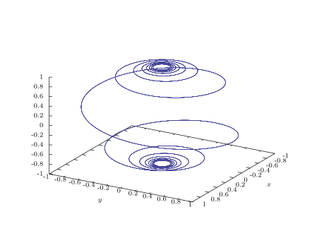
Figure 1.8.2 shows the graph of the curve when $a = 0.2$. In the exercises, the reader will be asked to show that this curve lies on the sphere $x^2 + y^2 + z^2 = 1$ and to verify directly that $\Dotprod{\textbf{f}\,'(t)}{\textbf{f}(t)} = 0$ for all $t$.

fig183 — Figure 1.8.2Spherical spiral with $a = 0.2$

width height 0.5pt Just as in single-variable calculus, higher-order derivatives of vector-valued functions are obtained by repeatedly differentiating the (first) derivative of the function:

\[\textbf{f}\,''(t) = \dfrac{d}{dt} \textbf{f}\,'(t) \; , \qquad \textbf{f}\,'''(t) = \dfrac{d}{dt} \textbf{f}\,''(t) \; , \quad \ldots \quad , \quad \dfrac{d^{n}\textbf{f}}{dt^{n}} = \dfrac{d}{dt} \biggl( \dfrac{d^{n-1}\textbf{f}}{dt^{n-1}} \biggr) \text{~~~(for $n = 2, 3, 4,\ldots$)}\]

We can use vector-valued functions to represent physical quantities, such as velocity, acceleration, force, momentum, etc. For example, let the real variable $t$ represent time elapsed from some initial time ($t = 0$), and suppose that an object of constant mass $m$ is subjected to some force so that it moves in space, with its position $(x,y,z)$ at time $t$ a function of $t$. That is, $x = x(t)$, $y = y(t)$, $z = z(t)$ for some real-valued functions $x(t)$, $y(t)$, $z(t)$. Call $\textbf{r}(t) = (x(t),y(t),z(t))$ the position vector of the object. We can define various physical quantities associated with the object as follows:^[1]

\begin{align*} \text{\emph{position}: } \textbf{r}(t) &= (x(t),y(t),z(t))\\ \text{\emph{velocity}: } \textbf{v}(t) &= \dot{\textbf{r}}(t) = \textbf{r}\,'(t) = \dfrac{d \textbf{r}}{dt}\\ &= (x'(t),y'(t),z'(t))\\ \text{\emph{acceleration}: } \textbf{a}(t) &= \dot{\textbf{v}}(t) = \textbf{v}\,'(t) = \dfrac{d \textbf{v}}{dt}\\ &= \ddot{\textbf{r}}(t) = \textbf{r}\,''(t) = \dfrac{d^2 \textbf{r}}{dt^2}\\ &= (x''(t),y''(t),z''(t))\\ \text{\emph{momentum}: } \textbf{p}(t) &= m \textbf{v}(t)\\ \text{\emph{force}: } \textbf{F}(t) &= \dot{\textbf{p}}(t) = \textbf{p}\,'(t) = \dfrac{d \textbf{p}}{dt} \text{~~~~(Newton's Second Law of Motion)} \end{align*}

The magnitude $\norm{\textbf{v}(t)}$ of the velocity vector is called the speed of the object. Note that since the mass $m$ is a constant, the force equation becomes the familiar $\textbf{F}(t) = m \textbf{a}(t)$.

width height 0.5pt

Example 1.39

Let $\textbf{r}(t) = (5 \cos t , 3 \sin t , 4 \sin t )$ be the position vector of an object at time $t \ge 0$. Find its (a) velocity and (b) acceleration vectors.

Solution: (a) $\textbf{v}(t) = \dot{\textbf{r}}(t) = (-5 \sin t , 3 \cos t , 4 \cos t )$

(b) $\textbf{a}(t) = \dot{\textbf{v}}(t) = (-5 \cos t , -3 \sin t , -4 \sin t )$

Note that $\norm{\textbf{r}(t)} = \sqrt{25 \cos^2 t + 25 \sin^2 t} = 5$ for all $t$, so by Example 1.37 we know that $\Dotprod{\textbf{r}(t)}{\dot{\textbf{r}}(t)} = 0$ for all $t$ (which we can verify from part (a)). In fact, $\norm{\textbf{v}(t)} = 5$ for all $t$ also. And not only does $\textbf{r}(t)$ lie on the sphere of radius $5$ centered at the origin, but perhaps not so obvious is that it lies completely within a circle of radius 5 centered at the origin. Also, note that $\textbf{a}(t) = -\textbf{r}(t)$. It turns out (see Exercise 16) that whenever an object moves in a circle with constant speed, the acceleration vector will point in the opposite direction of the position vector (i.e. towards the center of the circle).

width height 0.5pt Recall from Section 1.5 that if $\ssub{\textbf{r}}{1}$, $\ssub{\textbf{r}}{2}$ are position vectors to distinct points then $\ssub{\textbf{r}}{1} + t (\ssub{\textbf{r}}{2} - \ssub{\textbf{r}}{1})$ represents a line through those two points as $t$ varies over all real numbers. That vector sum can be written as $(1 - t) \ssub{\textbf{r}}{1} + t \ssub{\textbf{r}}{2}$. So the function $\textbf{l}(t) = (1 - t) \ssub{\textbf{r}}{1} + t \ssub{\textbf{r}}{2}$ is a line through the terminal points of $\ssub{\textbf{r}}{1}$ and $\ssub{\textbf{r}}{2}$, and when $t$ is restricted to the interval $\left[ 0,1 \right]$ it is the line segment between the points, with $\textbf{l}(0) = \ssub{\textbf{r}}{1}$ and $\textbf{l}(1) = \ssub{\textbf{r}}{2}$.

In general, a function of the form $\textbf{f}(t) = (\ssub{a}{1}t + \ssub{b}{1},\ssub{a}{2}t + \ssub{b}{2},\ssub{a}{3}t + \ssub{b}{3})$ represents a line in $\Real{3}$. A function of the form $\textbf{f}(t) = (\ssub{a}{1}t^2 + \ssub{b}{1}t + \ssub{c}{1},\ssub{a}{2}t^2 + \ssub{b}{2}t + \ssub{c}{2}, \ssub{a}{3}t^2 + \ssub{b}{3}t + \ssub{c}{3})$ represents a (possibly degenerate) parabola in $\Real{3}$.

width height 0.5pt

Example 1.40

Bézier curves are used in Computer Aided Design (CAD) to approximate the shape of a polygonal path in space (called the Bézier polygon or control polygon). For instance, given three points (or position vectors) $\ssub{\textbf{b}}{0}$, $\ssub{\textbf{b}}{1}$, $\ssub{\textbf{b}}{2}$ in $\Real{3}$, define

\begin{align*} \ssub{\textbf{b}}{0}^{\scriptscriptstyle 1}(t) &= ( 1 - t )\ssub{\textbf{b}}{0} + t \ssub{\textbf{b}}{1}\\ \ssub{\textbf{b}}{1}^{\scriptscriptstyle 1}(t) &= ( 1 - t )\ssub{\textbf{b}}{1} + t \ssub{\textbf{b}}{2}\\ \ssub{\textbf{b}}{0}^{\scriptscriptstyle 2}(t) &= ( 1 - t )\ssub{\textbf{b}}{0}^{\scriptscriptstyle 1}(t) + t \ssub{\textbf{b}}{1}^{\scriptscriptstyle 1}(t)\\ &= (1 - t)^2 \ssub{\textbf{b}}{0} + 2t(1 - t) \ssub{\textbf{b}}{1} + t^2 \ssub{\textbf{b}}{2} \end{align*}

for all real $t$. For $t$ in the interval $[0,1]$, we see that $\ssub{\textbf{b}}{0}^{\scriptscriptstyle 1}(t)$ is the line segment between $\ssub{\textbf{b}}{0}$ and $\ssub{\textbf{b}}{1}$, and $\ssub{\textbf{b}}{1}^{\scriptscriptstyle 1}(t)$ is the line segment between $\ssub{\textbf{b}}{1}$ and $\ssub{\textbf{b}}{2}$. The function $\ssub{\textbf{b}}{0}^{\scriptscriptstyle 2}(t)$ is the Bézier curve for the points $\ssub{\textbf{b}}{0}$, $\ssub{\textbf{b}}{1}$, $\ssub{\textbf{b}}{2}$. Note from the last formula that the curve is a parabola that goes through $\ssub{\textbf{b}}{0}$ (when $t = 0$) and $\ssub{\textbf{b}}{2}$ (when $t = 1$).

As an example, let $\ssub{\textbf{b}}{0} = (0,0,0)$, $\ssub{\textbf{b}}{1} = (1,2,3)$, and $\ssub{\textbf{b}}{2} = (4,5,2)$. Then the explicit formula for the Bézier curve is $\ssub{\textbf{b}}{0}^{\scriptscriptstyle 2}(t) = ( 2t + 2t^2, 4t + t^2, 6t - 4t^2 )$, as shown in Figure 1.8.3, where the line segments are $\ssub{\textbf{b}}{0}^{\scriptscriptstyle 1}(t)$ and $\ssub{\textbf{b}}{1}^{\scriptscriptstyle 1}(t)$, and the curve is $\ssub{\textbf{b}}{0}^{\scriptscriptstyle 2}(t)$.

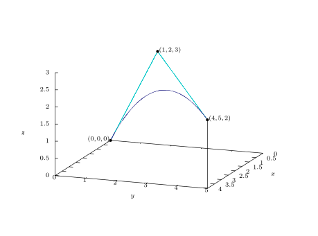
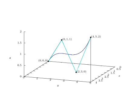
fig184 — Figure 1.8.3Bézier curve approximation for three points

In general, the polygonal path determined by $n \ge 3$ noncollinear points in $\Real{3}$ can be used to define the Bézier curve recursively by a process called repeated linear interpolation. This curve will be a vector-valued function whose components are polynomials of degree $n-1$, and its formula is given by de Casteljau’s algorithm.^[2] In the exercises, the reader will be given the algorithm for the case of $n = 4$ points and asked to write the explicit formula for the Bézier curve for the four points shown in Figure 1.8.4.

fig185 — Figure 1.8.4Bézier curve approximation for four points

Exercises

For Exercises 1-4, calculate $\textbf{f}\,'(t)$ and find the tangent line at $\textbf{f}(0)$.

$\textbf{f}(t) = (t + 1 , t^2 + 1 , t^3 + 1)$
$\textbf{f}(t) = (e^t + 1 , e^{2t} + 1 , e^{t^2} + 1)$

2
$\textbf{f}(t) = (\cos 2t , \sin 2t , t)$
$\textbf{f}(t) = (\sin 2t , 2\sin^2 t , 2\cos t)$

For Exercises 5-6, find the velocity $\textbf{v}(t)$ and acceleration $\textbf{a}(t)$ of an object with the given position vector $\textbf{r}(t)$.

$\textbf{r}(t) = (t, t - \sin t , 1 - \cos t)$
$\textbf{r}(t) = (3\cos t , 2\sin t , 1)$

Let $\textbf{f}(t) = \biggl( \dfrac{\cos t}{\sqrt{1 + a^2 t^2}},\dfrac{\sin t}{\sqrt{1 + a^2 t^2}}, \dfrac{-at}{\sqrt{1 + a^2 t^2}} \biggr)$, with $a \ne 0$.
1. Show that $\norm{\textbf{f}(t)} = 1$ for all $t$.
2. Show directly that $\Dotprod{\textbf{f}\,'(t)}{\textbf{f}(t)} = 0$ for all $t$.
If $\textbf{f}\,'(t) = \textbf{0}$ for all $t$ in some interval $(a,b)$, show that $\textbf{f}(t)$ is a constant vector in $(a,b)$.
For a constant vector $\textbf{c} \ne \textbf{0}$, the function $\textbf{f}(t) = t\textbf{c}$ represents a line parallel to $\textbf{c}$.
1. What kind of curve does $\textbf{g}(t) = t^3\textbf{c}$ represent? Explain.
2. What kind of curve does $\textbf{h}(t) = e^t\textbf{c}$ represent? Explain.
3. Compare $\textbf{f}\,'(0)$ and $\textbf{g}\,'(0)$. Given your answer to part (a), how do you explain the difference in the two derivatives?
Show that $\dfrac{d}{dt} \biggl( \Crossprod{\textbf{f}\,}{\dfrac{d\textbf{f}}{dt}} \biggr) = \Crossprod{\textbf{f}\,}{\dfrac{d^2 \textbf{f}}{dt^2}}\;$.
Let a particle of (constant) mass $m$ have position vector $\textbf{r}(t)$, velocity $\textbf{v}(t)$, acceleration $\textbf{a}(t)$ and momentum $\textbf{p}(t)$ at time $t$. The angular momentum $\textbf{L}(t)$ of the particle with respect to the origin at time $t$ is defined as $\textbf{L}(t) = \Crossprod{\textbf{r}(t)}{\,\textbf{p}(t)}$. If $\textbf{F}(t)$ is the force acting on the particle at time $t$, then define the torque $\textbf{N}(t)$ acting on the particle with respect to the origin as $\textbf{N}(t) = \Crossprod{\textbf{r}(t)}{\textbf{F}(t)}$. Show that $\textbf{L}\,'(t) = \textbf{N}(t)$.
Show that $\dfrac{d}{dt} ( \Dotprod{\textbf{f}}{( \Crossprod{\textbf{g}\,}{\,\textbf{h}} )} ) = \Dotprod{\dfrac{d\textbf{f}}{dt}}{(\Crossprod{\textbf{g}\,}{\,\textbf{h}})} \,+\, \Dotprod{\textbf{f}}{\biggl(\Crossprod{\dfrac{d \textbf{g}}{dt}}{\,\textbf{h}}\biggr)} \,+\, \Dotprod{\textbf{f}}{\biggl(\Crossprod{\textbf{g}\,}{\dfrac{d \textbf{h}}{dt}}\biggr)}$.
The Mean Value Theorem does not hold for vector-valued functions: Show that for $\textbf{f}(t) = (\cos t, \sin t,t)$, there is no $t$ in the interval $(0,2\pi)$ such that

\[ \textbf{f}\,'(t) = \dfrac{\textbf{f}(2\pi) - \textbf{f}(0)}{2\pi - 0} . \]

The Bézier curve $\ssub{\textbf{b}}{0}^{\scriptscriptstyle 3}(t)$ for four noncollinear points $\ssub{\textbf{b}}{0}$, $\ssub{\textbf{b}}{1}$, $\ssub{\textbf{b}}{2}$, $\ssub{\textbf{b}}{3}$ in $\Real{3}$ is defined by the following algorithm (going from the left column to the right):

\begin{alignat*}{3} \ssub{\textbf{b}}{0}^{\scriptscriptstyle 1}(t) &= ( 1 - t )\ssub{\textbf{b}}{0} + t \ssub{\textbf{b}}{1} \qquad & \ssub{\textbf{b}}{0}^{\scriptscriptstyle 2}(t) &= ( 1 - t )\ssub{\textbf{b}}{0}^{\scriptscriptstyle 1}(t) + t \ssub{\textbf{b}}{1}^{\scriptscriptstyle 1}(t) \qquad & \ssub{\textbf{b}}{0}^{\scriptscriptstyle 3}(t) &= ( 1 - t )\ssub{\textbf{b}}{0}^{\scriptscriptstyle 2}(t) + t \ssub{\textbf{b}}{1}^{\scriptscriptstyle 2}(t)\\ \ssub{\textbf{b}}{1}^{\scriptscriptstyle 1}(t) &= ( 1 - t )\ssub{\textbf{b}}{1} + t \ssub{\textbf{b}}{2} \qquad & \ssub{\textbf{b}}{1}^{\scriptscriptstyle 2}(t) &= ( 1 - t )\ssub{\textbf{b}}{1}^{\scriptscriptstyle 1}(t) + t \ssub{\textbf{b}}{2}^{\scriptscriptstyle 1}(t)\\ \ssub{\textbf{b}}{2}^{\scriptscriptstyle 1}(t) &= ( 1 - t )\ssub{\textbf{b}}{2} + t \ssub{\textbf{b}}{3} \end{alignat*}
1. Show that $\ssub{\textbf{b}}{0}^{\scriptscriptstyle 3}(t) = (1 - t)^3 \ssub{\textbf{b}}{0} + 3t(1 - t)^2 \ssub{\textbf{b}}{1} + 3t^2 (1 - t) \ssub{\textbf{b}}{2} + t^3 \ssub{\textbf{b}}{3}$.
2. Write the explicit formula (as in Example 1.40) for the Bézier curve for the points $\ssub{\textbf{b}}{0} = (0,0,0)$, $\ssub{\textbf{b}}{1} = (0,1,1)$, $\ssub{\textbf{b}}{2} = (2,3,0)$, $\ssub{\textbf{b}}{3} = (4,5,2)$.
Let $\textbf{r}(t)$ be the position vector for a particle moving in $\Real{3}$. Show that

\[ \dfrac{d}{dt} ( \Crossprod{\textbf{r}}{( \Crossprod{\textbf{v}\,}{\,\textbf{r}} )} ) = \norm{\textbf{r}}^2 \textbf{a} + (\Dotprod{\textbf{r}}{\textbf{v}}) \textbf{v} - (\norm{\textbf{v}}^2 + \Dotprod{\textbf{r}}{\textbf{a}})\textbf{r} . \]
Let $\textbf{r}(t)$ be the position vector in $\Real{3}$ for a particle moving at constant speed $c > 0$ in a circle of radius $a > 0$ in the $xy$-plane. Show that $\textbf{a}(t)$ points in the opposite direction as $\textbf{r}(t)$ for all $t$. (Hint: Use Example 1.37 to show that $\textbf{r}(t) \perp \textbf{v}(t)$ and $\textbf{a}(t) \perp \textbf{v}(t)$).
Prove Theorem 1.20(g).

We will often use the older dot notation for derivatives when physics is involved. ↩
See pp. 27-30 in far. ↩