In single-variable calculus, the functions that one encounters are functions of a variable (usually \(x\) or \(t\)) that varies over some subset of the real number line (which we denote by \(\mathbb{R}\)). For such a function, say, \(y = f(x)\), the graph of the function \(f\) consists of the points \((x, y) = (x, f(x))\). These points lie in the Euclidean plane, which, in the Cartesian or rectangular coordinate system, consists of all ordered pairs of real numbers \((a, b)\). We use the word “Euclidean” to denote a system in which all the usual rules of Euclidean geometry hold. We denote the Euclidean plane by \(\Real{2}\); the “2” represents the number of dimensions of the plane. The Euclidean plane has two perpendicular coordinate axes: the \(x\)-axis and the \(y\)-axis.
In vector (or multivariable) calculus, we will deal with functions of two or three variables (usually \(x, y\) or
\(x, y, z\), respectively). The graph of a function of two variables, say, \(z = f(x,y)\), lies in
Euclidean space, which in the Cartesian coordinate system consists of all ordered
triples of real numbers \((a, b, c)\). Since Euclidean space is 3-dimensional, we denote it by
\(\Real{3}\). The graph of \(f\) consists
of the points \((x, y, z) = (x, y, f(x, y))\). The 3-dimensional coordinate system of Euclidean space can be
represented on a flat surface, such as this page or a blackboard, only by giving the illusion of three
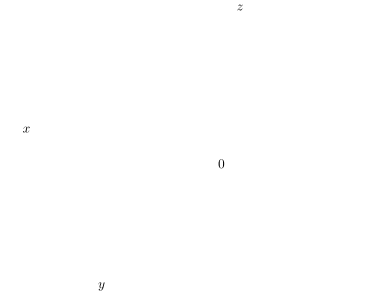
dimensions, in the manner shown in Figure 1.1.1. Euclidean space has three mutually perpendicular
coordinate axes (\(x, y\) and \(z\)), and three mutually perpendicular coordinate planes:
the \(xy\)-plane, \(yz\)-plane and \(xz\)-plane (see Figure 1.1.2).


The coordinate system shown in Figure 1.1.1 is known as a right-handed coordinate system, because it is possible, using the right hand, to point the index finger in the positive direction of the \(x\)-axis, the middle finger in the positive direction of the \(y\)-axis, and the thumb in the positive direction of the \(z\)-axis, as in Figure 1.1.3.
An equivalent way of defining a right-handed system is if you can point your thumb upwards in the positive \(z\)-axis direction while using the remaining four fingers to rotate the \(x\)-axis towards the \(y\)-axis. Doing the same thing with the left hand is what defines a left-handed coordinate system. Notice that switching the \(x\)- and \(y\)-axes in a right-handed system results in a left-handed system, and that rotating either type of system does not change its “handedness”. Throughout the book we will use a right-handed system.
For functions of three variables, the graphs exist in 4-dimensional space (i.e. \(\Real{4}\)), which we can not see in our 3-dimensional space, let alone simulate in 2-dimensional space. So we can only think of 4-dimensional space abstractly. For an entertaining discussion of this subject, see the book by abb.[1]
So far, we have discussed the position of an object in 2-dimensional or 3-dimensional space. But what about something such as the velocity of the object, or its acceleration? Or the gravitational force acting on the object? These phenomena all seem to involve motion and direction in some way. This is where the idea of a vector comes in. You have already dealt with velocity and acceleration in single-variable calculus. For example, for motion along a straight line, if \(y = f(t)\) gives the displacement of an object after time \(t\), then \(dy/dt = f\,'(t)\) is the velocity of the object at time \(t\). The derivative \(f\,'(t)\) is just a number, which is positive if the object is moving in an agreed-upon “positive” direction, and negative if it moves in the opposite of that direction. So you can think of that number, which was called the velocity of the object, as having two components: a magnitude, indicated by a nonnegative number, preceded by a direction, indicated by a plus or minus symbol (representing motion in the positive direction or the negative direction, respectively), i.e. \(f\,'(t) = \pm a\) for some number \(a \ge 0\). Then \(a\) is the magnitude of the velocity (normally called the speed of the object), and the \(\pm\) represents the direction of the velocity (though the \(+\) is usually omitted for the positive direction).
For motion along a straight line, i.e. in a 1-dimensional space, the velocities are also contained in that 1-dimensional space, since they are just numbers. For general motion along a curve in 2- or 3-dimensional space, however, velocity will need to be represented by a multidimensional object which should have both a magnitude and a direction. A geometric object which has those features is an arrow, which in elementary geometry is called a “directed line segment”. This is the motivation for how we will define a vector.
Definition 1.1
A (nonzero) vector is a directed line segment drawn from a point \(P\) (called its initial point) to a point \(Q\) (called its terminal point), with \(P\) and \(Q\) being distinct points. The vector is denoted by \(\overrightarrow{PQ}\). Its magnitude is the length of the line segment, denoted by \(\Norm{\overrightarrow{PQ}}\), and its direction is the same as that of the directed line segment. The zero vector is just a point, and it is denoted by \(\textbf{0}\).
To indicate the direction of a vector, we draw an arrow from its initial point to its terminal point. We will often denote a vector by a single bold-faced letter (e.g. \(\textbf{v}\)) and use the terms “magnitude” and “length” interchangeably. Note that our definition could apply to systems with any number of dimensions (see Figure 1.1.4 (a)-(c)).


A few things need to be noted about the zero vector. Our motivation for what a vector is included the notions of magnitude and direction. What is the magnitude of the zero vector? We define it to be zero, i.e. \(\norm{\textbf{0}} = 0\). This agrees with the definition of the zero vector as just a point, which has zero length. What about the direction of the zero vector? A single point really has no well-defined direction. Notice that we were careful to only define the direction of a nonzero vector, which is well-defined since the initial and terminal points are distinct. Not everyone agrees on the direction of the zero vector. Some contend that the zero vector has arbitrary direction (i.e. can take any direction), some say that it has indeterminate direction (i.e. the direction can not be determined), while others say that it has no direction. Our definition of the zero vector, however, does not require it to have a direction, and we will leave it at that.[2]
Now that we know what a vector is, we need a way of determining when two vectors are equal. This leads us to the following definition.
Definition 1.2
Two nonzero vectors are equal if they have the same magnitude and the same direction. Any vector with zero magnitude is equal to the zero vector.
By this definition, vectors with the same magnitude and direction but with different initial points would be equal. For example, in Figure 1.1.5 the vectors u, v and w all have the same magnitude \(\sqrt 5\) (by the Pythagorean Theorem). And we see that u and w are parallel, since they lie on lines having the same slope \(\frac{1}{2}\), and they point in the same direction. So \(\textbf{u} = \textbf{w}\), even though they have different initial points. We also see that v is parallel to u but points in the opposite direction. So \(\textbf{u} \ne \textbf{v}\).

So we can see that there are an infinite number of vectors for a given magnitude and direction, those vectors all being equal and differing only by their initial and terminal points. Is there a single vector which we can choose to represent all those equal vectors? The answer is yes, and is suggested by the vector w in Figure 1.1.5.
Thinking of vectors as starting from the origin provides a way of dealing with vectors in a standard way, since every coordinate system has an origin. But there will be times when it is convenient to consider a different initial point for a vector (for example, when adding vectors, which we will do in the next section).
Another advantage of using the origin as the initial point is that it provides an easy correspondence between a vector and its terminal point.
width height 0.5pt
Example 1.1
Let v be the vector in \(\Real{3}\) whose initial point is at the origin and whose terminal point is \((3,4,5)\). Though the point \((3,4,5)\) and the vector v are different objects, it is convenient to write \(\textbf{v} = (3,4,5)\). When doing this, it is understood that the initial point of \(\textbf{v}\) is at the origin \((0,0,0)\) and the terminal point is \((3,4,5)\).


width height 0.5pt
Unless otherwise stated, when we refer to vectors as \(\textbf{v} = (a,b)\) in \(\Real{2}\) or \(\textbf{v} = (a,b,c)\) in \(\Real{3}\), we mean vectors in Cartesian coordinates starting at the origin. Also, we will write the zero vector \(\textbf{0}\) in \(\Real{2}\) and \(\Real{3}\) as \((0,0)\) and \((0,0,0)\), respectively.
The point-vector correspondence provides an easy way to check if two vectors are equal, without having to determine their magnitude and direction. Similar to seeing if two points are the same, you are now seeing if the terminal points of vectors starting at the origin are the same. For each vector, find the (unique!) vector it equals whose initial point is the origin. Then compare the coordinates of the terminal points of these “new” vectors: if those coordinates are the same, then the original vectors are equal. To get the “new” vectors starting at the origin, you translate each vector to start at the origin by subtracting the coordinates of the original initial point from the original terminal point. The resulting point will be the terminal point of the “new” vector whose initial point is the origin. Do this for each original vector then compare.
Example 1.2
Consider the vectors \(\overrightarrow{PQ}\) and \(\overrightarrow{RS}\) in \(\Real{3}\), where \(P = (2,1,5),
Q = (3,5,7), R = (1,-3,-2)\) and \(S = (2,1,0)\). Does \(\overrightarrow{PQ} =
\overrightarrow{RS}\)?
Solution:
The vector \(\overrightarrow{PQ}\) is equal to the vector v with
initial point \((0,0,0)\) and terminal point \(Q - P = (3,5,7) - (2,1,5) = (3 - 2,5 - 1,7 - 5) = (1,4,2)\).
Similarly, \(\overrightarrow{RS}\) is equal to the vector w with initial point \((0,0,0)\) and terminal point \(S - R = (2,1,0) - (1,-3,-2) = (2 - 1, 1 - (-3),0 - (-2)) = (1,4,2)\).
So \(\overrightarrow{PQ} = \textbf{v} = (1,4,2)\) and \(\overrightarrow{RS} = \textbf{w} = (1,4,2)\).
\(\therefore \overrightarrow{PQ} = \overrightarrow{RS}\)

width height 0.5pt
Recall the distance formula for points in the Euclidean plane:
For points \(P = (\ssub{x}{1},\ssub{y}{1})\), \(Q = (\ssub{x}{2},\ssub{y}{2})\) in \(\Real{2}\), the distance \(d\) between \(P\) and \(Q\) is:
By this formula, we have the following result:
For a vector \(\overrightarrow{PQ}\) in \(\Real{2}\) with initial point
\(P = (\ssub{x}{1},\ssub{y}{1})\) and terminal point
\(Q = (\ssub{x}{2},\ssub{y}{2})\), the magnitude of \(\overrightarrow{PQ}\) is:
Finding the magnitude of a vector \(\textbf{v} = (a,b)\) in \(\Real{2}\) is a special case of formula (1.2) with \(P = (0,0)\) and \(Q = (a,b)\) :
For a vector \(\textbf{v} = (a,b)\) in \(\Real{2}\), the magnitude of v is:
To calculate the magnitude of vectors in \(\Real{3}\), we need a distance formula for points in Euclidean space (we will postpone the proof until the next section):
Theorem 1.1
The distance \(d\) between points \(P = (\ssub{x}{1},\ssub{y}{1},\ssub{z}{1})\) and \(Q = (\ssub{x}{2},\ssub{y}{2},\ssub{z}{2})\) in \(\Real{3}\) is:
The proof will use the following result:
Theorem 1.2
For a vector \(\textbf{v} = (a,b,c)\) in \(\Real{3}\), the magnitude of v is:
proof[Proof:] There are four cases to consider:
Case 1: \(a = b = c = 0\). Then \(\textbf{v} = \textbf{0}\), so \(\norm{\textbf{v}} = 0 = \sqrt{0^2 + 0^2 + 0^2} = \sqrt{a^2 + b^2 + c^2}\).
Case 2: exactly two of \(a, b, c\) are \(0\). Without loss of generality, we assume that \(a = b = 0\) and \(c \ne 0\) (the other two possibilities are handled in a similar manner). Then \(\textbf{v} = (0,0,c)\), which is a vector of length \(\abs{c}\) along the \(z\)-axis. So \(\norm{\textbf{v}} = | c | = \sqrt{c^2} = \sqrt{0^2 + 0^2 + c^2} = \sqrt{a^2 + b^2 + c^2}\).
Case 3: exactly one of \(a, b, c\) is \(0\). Without loss of generality, we assume that \(a = 0\), \(b \ne 0\) and \(c \ne 0\) (the other two possibilities are handled in a similar manner). Then \(\textbf{v} = (0,b,c)\), which is a vector in the \(yz\)-plane, so by the Pythagorean Theorem we have \(\norm{\textbf{v}} = \sqrt{b^2 + c^2} = \sqrt{0^2 + b^2 + c^2} = \sqrt{a^2 + b^2 + c^2}\).

Case 4: none of \(a, b, c\) are \(0\). Without loss of generality, we can assume that
\(a, b, c\) are all positive (the other seven possibilities are handled in a similar manner).
Consider the points \(P = (0,0,0)\), \(Q = (a,b,c)\), \(R =(a,b,0),\) and \(S = (a,0,0)\), as shown in Figure 1.1.8. Applying
the Pythagorean Theorem to the right triangle \(\triangle PSR\) gives \(\left\vert PR \right\vert^2 = a^2 + b^2\). A second
application of the Pythagorean Theorem, this time to the right triangle \(\triangle PQR\), gives \(\norm{\textbf{v}}
= \left\lvert PQ \right\rvert = \sqrt{\left\vert PR \right\vert^2 + \left\vert QR \right\vert^2} =
\sqrt{a^2 + b^2 + c^2}\).
This proves the theorem.
Example 1.3
Calculate the following:
The magnitude of the vector \(\overrightarrow{PQ}\) in \(\Real{2}\) with \(P = (-1,2)\) and \(Q = (5,5)\).
Solution: By formula (1.2), \(\Norm{\overrightarrow{PQ}} = \sqrt{(5 - (-1))^2 + (5 - 2)^2} = \sqrt{36 + 9} = \sqrt{45} = 3 \sqrt{5}\).The magnitude of the vector \(\textbf{v} = (8,3)\) in \(\Real{2}\).
Solution: By formula (1.3), \(\norm{\textbf{v}} = \sqrt{8^2 + 3^2} = \sqrt{73}\).The distance between the points \(P = (2, -1, 4)\) and \(Q = (4, 2, -3)\) in \(\Real{3}\).
Solution: By formula (1.4), the distance \(d = \sqrt{(4 - 2)^2 + (2 - (-1))^2 + (-3 - 4)^2} =\)
\(\sqrt{4 + 9 + 49} = \sqrt{62}\).The magnitude of the vector \(\textbf{v} = (5,8,-2)\) in \(\Real{3}\).
Solution: By formula (1.5), \(\norm{\textbf{v}} = \sqrt{5^2 + 8^2 + (-2)^2} = \sqrt{25 + 64 + 4} = \sqrt{93}\).
A
Calculate the magnitudes of the following vectors:
(a) \(\textbf{v} = (2,-1)\) (b) \(\textbf{v} = (2,-1,0)\) (c) \(\textbf{v} = (3,2,-2)\) (d) \(\textbf{v} = (0,0,1)\) (e) \(\textbf{v} = (6,4,-4)\) For the points \(P =(1,-1,1)\), \(Q=(2,-2,2)\), \(R=(2,0,1)\), \(S=(3,-1,2)\), does \(\overrightarrow{PQ} = \overrightarrow{RS}\)?
For the points \(P =(0,0,0)\), \(Q=(1,3,2)\), \(R=(1,0,1)\), \(S=(2,3,4)\), does \(\overrightarrow{PQ} = \overrightarrow{RS}\)?
B
Let \(\textbf{v} = (1,0,0)\) and \(\textbf{w} = (a,0,0)\) be vectors in \(\Real{3}\). Show that \(\norm{\textbf{w}} = \abs{a} \,\norm{\textbf{v}}\).
Let \(\textbf{v} = (a,b,c)\) and \(\textbf{w} = (3a,3b,3c)\) be vectors in \(\Real{3}\). Show that \(\norm{\textbf{w}} = 3 \,\norm{\textbf{v}}\).
C

Though we will see a simple proof of Theorem 1.1 in the next section, it is possible to prove it using methods similar to those in the proof of Theorem 1.2. Prove the special case of Theorem 1.1 where the points \(P = (\ssub{x}{1},\ssub{y}{1},\ssub{z}{1})\) and \(Q = (\ssub{x}{2},\ssub{y}{2},\ssub{z}{2})\) satisfy the following conditions:
\(\ssub{x}{2} > \ssub{x}{1} > 0\), \(\ssub{y}{2} > \ssub{y}{1} > 0\), and \(\ssub{z}{2} > \ssub{z}{1} > 0\).
(Hint: Think of Case 4 in the proof of Theorem 1.2, and consider Figure 1.1.9.)
Unless otherwise indicated, when speaking of “the vector” with a given magnitude and direction, we will mean the one whose initial point is at the origin of the coordinate system.