4.2 Curve Sketching

A function can increase between two points in different ways, as shown in Figure 4.2.1.

tikzpicture[>=latex,every node/.style=font=] [black!60,line width=1pt,<->] (0,3) node[above] y |- (3,0) node[right] x; [linecolor,line width=1.5pt] (0.5,0.5) -- (2.5,2.5) node[black,pos=0.6,above left] y = f(x); (0.5,0.5) circle (2.5pt); (2.5,2.5) circle (2.5pt); tikzpicture — Figure 4.2.1Increasing function $f$: $f'>0$, different signs for $f''$

tikzpicture[>=latex,every node/.style=font=] [black!60,line width=1pt,<->] (0,3) node[above] y |- (3,0) node[right] x; [linecolor,line width=1.5pt] (0.5,0.5) parabola (2.5,2.5); [left] at (2,2.5) y = f(x); (0.5,0.5) circle (2.5pt); (2.5,2.5) circle (2.5pt); tikzpicture — Figure 4.2.1Increasing function $f$: $f'>0$, different signs for $f''$

In each case in the above figure the function is increasing, so that $f'(x) > 0$, but the manner in which the function increases is determined by its concavity, that is, by the sign of the second derivative $f''(x)$. The function in the graph on the far left is linear, i.e. of the form $f(x) = ax+b$ for some constants $a$ and $b$, so that $f''(x)=0$ for all $x$. But the functions in the other two graphs are nonlinear. In the middle graph the derivative $f'$ is increasing, so that $f''>0$; in this case the function is called concave up. In the graph on the far right the derivative $f'$ is decreasing, so that $f''<0$; in this case the function is called concave down. The same definitions would hold if the function were decreasing, as shown in Figure 4.2.2 below:

tikzpicture[>=latex,every node/.style=font=] [black!60,line width=1pt,<->] (0,3) node[above] y |- (3,0) node[right] x; [linecolor,line width=1.5pt] (0.5,2.5) -- (2.5,0.5) node[black,pos=0.6,above right] y = f(x); (0.5,2.5) circle (2.5pt); (2.5,0.5) circle (2.5pt); tikzpicture — Figure 4.2.2Decreasing function $f$: $f'<0$, different signs for $f''$

tikzpicture[>=latex,every node/.style=font=] [black!60,line width=1pt,<->] (0,3) node[above] y |- (3,0) node[right] x; [linecolor,line width=1.5pt] (0.5,2.5) parabola[bend at end] (2.5,0.5); [right] at (1.3,2.5) y = f(x); (0.5,2.5) circle (2.5pt); (2.5,0.5) circle (2.5pt); tikzpicture — Figure 4.2.2Decreasing function $f$: $f'<0$, different signs for $f''$

In Figures 4.2.1(b) and 4.2.2(b) the function is below the line joining the points at each end, while in Figure 4.2.1(c) and 4.2.2(c) the function is above that line. This turns out to be true in general, as a result of the following theorem:

Theorem 4.2

Concavity Theorem: Suppose that $f$ is a twice-differentiable function on $\ival{a}{b}$. Then:

If $f''(x)>0$ on $(a,b)$ then $f(x)$ is below the line $l(x)$ joining the points $(a,f(a))$ and $(b,f(b))$ for all $x$ in $(a,b)$.
If $f''(x)<0$ on $(a,b)$ then $f(x)$ is above the line $l(x)$ joining the points $(a,f(a))$ and $(b,f(b))$ for all $x$ in $(a,b)$.

[r] Proof: Only part (a) will be proved; the proof of part (b) is similar and left as an exercise. So assume that $f''(x)>0$ on $(a,b)$, and $l(x)$ be the line joining $(a,f(a))$ and $(b,f(b))$, as in the drawing on the right. The drawing suggests that $f(x)$ < $l(x)$ over $(a,b)$, but this is what must be proved.

The goal is to show that $g(x) = f(x) - l(x) < 0$ on $(a,b)$, since this will show that $f(x) < l(x)$ on $(a,b)$. Since $f$ and $l$ are both continuous on $\ival{a}{b}$ then so is $g$. Hence $g$ has a global maximum somewhere in $\ival{a}{b}$, by the Extreme Value Theorem. Suppose the global maximum occurs at an interior point $x=c$, i.e. for some $c$ in the open interval $(a,b)$. Then $g'(c)=0$ and $g''(c)=f''(c)-l''(c)=f''(c)>0$, since $l(x)$ is a line and hence has a second derivative of $0$ for all $x$. Then by the Second Derivative Test $g$ has a local minimum at $x=c$, which contradicts $g$ having a global maximum at $x=c$. Thus, the global maximum of $g$ cannot occur at an interior point, so it must occur at one of the end points $x=a$ or $x=b$. In other words, either $g(x)<g(a)$ or $g(x)<g(b)$ for all $x$ in $(a,b)$. But $f(a)=l(a)$ and $f(b)=l(b)$, so $g(a)=0=g(b)$. Hence, $g(x)<0$ for all $x$ in $(a,b)$, i.e. $f(x) < l(x)$ for all $x$ in $(a,b). \quad\checkmark$

Points where the concavity of a function changes have a special name:

Definition 4.1

A function $f$ has an inflection point at $x=c$ if the concavity of $f$ changes around $x=c$. That is, the function goes from concave up to concave down, or vice versa.

Note that to be an inflection point it does not suffice for the second derivative to be 0 at that point; the second derivative must change sign around that point, either from positive to negative or from negative to positive. For example, $f(x) = x^3$ has an inflection point at $x=0$, since $f''(x)=6x<0$ for $x<0$ and $f''(x)=6x>0$ for $x>0$, i.e. $f''(x)$ changes sign around $x=0$ (and of course $f''(0)=0$). But for $f(x)=x^4$, $x=0$ is not an inflection point even though $f''(0)=0$, since $f''(x)=12x^2\ge 0$ is always nonnegative. That is, $f(x)=x^4$ is always concave up. Figure 4.2.3 below shows the difference:

tikzpicture[>=latex,every node/.style=font=] [black!60,line width=1pt,->] (0,-1) -- (0,1) node[above] y; [black!60,line width=1pt,->] (-1.5,0) -- (1.5,0) node[right] x; [linecolor,line width=1.5pt] (-1.5,-1) parabola[bend at end] (0,0); [linecolor,line width=1.5pt] (0,0) parabola (1.5,1); (0,0) circle (2.5pt); [below right] at (0,0) 0; [white] (-3,1) -- (-2,1); [white] (2,1) -- (3,1); tikzpicture — Figure 4.2.3Inflection vs non-inflection point at $x=0$ with $f''(0)=0$

tikzpicture[>=latex,every node/.style=font=] [black!60,line width=1pt,->] (0,0) -- (0,2) node[above] y; [black!60,line width=1pt,->] (-1.5,0) -- (1.5,0) node[right] x; [linecolor,line width=1.5pt] (-1.5,2) parabola bend (0,0) (1.5,2); (0,0) circle (2.5pt); [below] at (0,0) 0; [white] (-3.5,1) -- (-2,1); [white] (2,1) -- (3.5,1); tikzpicture — Figure 4.2.3Inflection vs non-inflection point at $x=0$ with $f''(0)=0$

Figure 4.2.3(b) shows that a point where the second derivative is 0 is a possible inflection point, but you still must check that the second derivative changes sign around that point. Using local minima and maxima, concavity and inflection points, and where a function increases or decreases, you can sketch the graph of a function.

Example 4.8

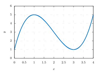
Sketch the graph of $f(x) ~=~ x^3 ~-~ 6x^2 ~+~ 9x ~+~ 1$. Find all local maxima and minima, inflection points, where the function is increasing or decreasing, and where the function is concave up or concave down.

Solution: Since $f'(x) = 3x^2 - 12x + 9 ~=~ 3\,(x-1)\,(x-3)$ then $x=1$ and $x=3$ are the only critical points. And since $f''(x) = 6x-12$ then $f''(1) = -6 < 0$ and $f''(3) = 6 > 0$. So by the Second Derivative Test, $f$ has a local maximum at $x=1$ and a local minimum at $x=3$. Since $f''(x) = 6x-12 < 0$ for $x<2$ and $f''(x) = 6x-12 > 0$ for $x>2$, then $x=2$ is an inflection point, and $f$ is concave down for $x <2$ and concave up for $x>2$. The table below shows where $f$ is increasing and decreasing, based on the sign of $f'$:

$x$ values	$3\,(x-1)$	$(x-3)$	$f'(x)$	direction
$x < 1$	$-$	$-$	$+$	$f$ is increasing
$1 < x < 3$	$+$	$-$	$-$	$f$ is decreasing
$x > 3$	$+$	$+$	$+$	$f$ is increasing

The graph is shown below:

calc12ex48

Example 4.9

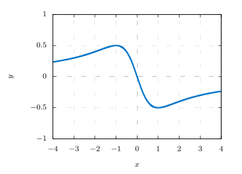
Sketch the graph of $f(x) ~=~ \frac{-x}{1 ~+~ x^2}$. Find all local maxima and minima, inflection points, where the function is increasing or decreasing, and where the function is concave up or concave down. Also indicate any asymptotes.

Solution: Since $f'(x) = \frac{x^2 - 1}{(1+x^2)^2}$ then $x=1$ and $x=-1$ are the only critical points. And since $f''(x) = \frac{2x\,(3 - x^2)}{(1+x^2)^3}$ then $f''(1) = \frac{1}{2} > 0$ and $f''(-1) = -\frac{1}{2} < 0$. So by the Second Derivative Test, $f$ has a local minimum at $x=1$ and a local maximum at $x=-1$. Since $f''(x) > 0$ for $x<-\sqrt{3}$, $f''(x) < 0$ for $-\sqrt{3}<x<0$, $f''(x) > 0$ for $0<x<\sqrt{3}$, and $f''(x) < 0$ for $x>\sqrt{3}$, then $x=0,\pm\sqrt{3}$ are inflection points, $f$ is concave up for $x<-\sqrt{3}$ and for $0<x<\sqrt{3}$, and $f$ is concave down for $-\sqrt{3}<x<0$ and for $x>\sqrt{3}$. Since $f'(x)>0$ for $x<-1$ and $x>1$ then $f$ is increasing for $\abs{x} > 1$. And $f'(x)<0$ for $-1<x<1$ means $f$ is decreasing for $\abs{x}<1$. Finally, since $\displaystyle\lim_{x \to \infty} f(x) = 0$ and $\displaystyle\lim_{x \to -\infty} f(x) = 0$ then the $x$-axis ($y=0$) is a horizontal asymptote. There are no vertical asymptotes (why?).

The graph is shown below:

calc12ex49

If the Second Derivative Test fails then one alternative is the following test:

Theorem 4.3

First Derivative Test: For a continuous function $f$ on an interval $I$, let $x=c$ be a number in $I$ such that $f(c)$ is defined, and either $f'(c)=0$ or $f'(c)$ does not exist. Then:

If $f'(x)$ changes from negative to positive around $x=c$ then $f$ has a local minimum at $x=c$.
If $f'(x)$ changes from positive to negative around $x=c$ then $f$ has a local maximum at $x=c$.

This test merely states the obvious: a function decreases then increases around a minimum, and it increases then decreases around a maximum.

Example 4.10

[r]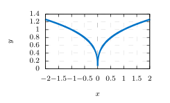 calc12ex410 Sketch the graph of $f(x) = x^{2/3}$.

Solution: Clearly $f(x)$ is continuous for all $x$, including $x=0$ (since $f(0)=0$), but $f'(x) = \frac{2}{3\,\sqrt[3]{x}}$ is not defined at $x=0$. Since $f'(x)$ changes from negative to positive around $x=0$ ($f'(x) < 0$ when $x < 0$ and $f'(x) > 0$ when $x > 0$), then by the First Derivative Test $f$ has a local minimum at $x=0$. Since $f''(x) = -\, \frac{2}{9\,x^{4/3}} < 0$ for all $x \ne 0$, then $f$ is always concave down. There are no vertical or horizontal asymptotes. The graph is shown on the right.

Note that the Second Derivative Test could not be used for this function, since $f'(x) \ne 0$ for all $x$ (notice also that $f''(x)$ is not defined at $x=0$).

A more complete alternative to the Second Derivative Test is the following:^[1]

Theorem 4.4

N^th Derivative Test: A non-constant function $f$ with continuous derivatives of all orders up to and including $n >1$ at $x=c$ has either a local minimum, local maximum or inflection point at $x=c$ if and only if

\[ f^{(k)}(c) ~=~ 0 ~~\text{for $k=1$, $2$, $\ldots$, $n-1$} \quad\text{and}\quad f^{(n)}(c) ~\ne~ 0 \]

(i.e. the $n^{\text{th}}$ derivative is the first nonzero derivative at $x=c$). If so, then:

If $n>1$ is even and $f^{(n)}(c) > 0$ then $f$ has a local minimum at $x=c$.
If $n>1$ is even and $f^{(n)}(c) < 0$ then $f$ has a local maximum at $x=c$.
If $n>1$ is odd then $f$ has an inflection point at $x=c$.

Note that the Second Derivative Test is the special case where $n=2$ in the N^th Derivative Test. Though this test gives necessary and sufficient conditions for a local maximum, local minimum, and inflection point, calculating the first $n$ derivatives can be complicated if $n$ is large and the given function is not simple.

Example 4.11

The Second Derivative Test fails for $f(x)=x^4$ at the critical point $x=0$, since $f''(0)=0$. But the first 4 derivatives of $f(x)=x^4$ are $f'(x)=4x^3$, $f''(x)=12x^2$, $f^{(3)}(x)=24x$, and $f^{(4)}(x)=24$, which are all continuous and

\[ f^{(k)}(0) ~=~ 0 ~~\text{for $k=1$, $2$, $3$} \quad\text{and}\quad f^{(4)}(0) ~=~ 24 ~\ne~ 0 ~. \]

So by the N^th Derivative Test, since $n=4$ is even and $f^{(4)}(0)=24>0$ then $f(x)=x^4$ has a local minimum at $x=0$. Note that $f(x) \ge 0 = f(0)$ for all $x$, so $x = 0$ is actually a global minimum for $f$.

A common practice in many fields of science and engineering is to combine multiple named constants (e.g. $\pi$) or variables in a function into one variable and then sketch a graph of that function. The example below illustrates the technique.

Example 4.12

A hydrogen atom has one electron, and the probability of finding the electron in the ground state of the hydrogen atom between radii $r$ and $r+\dr$ is $D(r)\,\dr$, where $\dr$ is an infinitesimal change in the radius $r$ (the distance from the electron to the nucleus), $D(r)$ is the radial probability density function

\[ D(r) ~=~ \frac{4}{a_0^3}\,r^2 e^{-2r/a_0} \]

and $a_0 \approx 5.291772 \times 10^{-11}$ m is the Bohr radius. It is useful to analyze this function in terms of $r \ge 0$ in relation to the Bohr radius $a_0$ (e.g. $r= 0.5a_0$, $a_0$, $2a_0$, $3a_0$). To do this, let $x = \frac{r}{a_0}$, so that

\[ D(r) ~=~ \frac{4}{a_0}\,\left(\frac{r}{a_0}\right)^2 e^{-2\left(\frac{r}{a_0}\right)} \quad\Rightarrow\quad a_0\,D(x) ~=~ 4x^2 e^{-2x} \]

and then sketch the graph of $a_0\,D(x)$, which is shown below:

calc12ex412

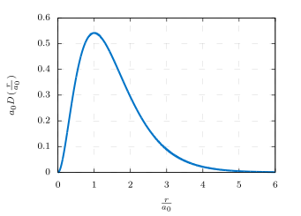
From the graph it looks like $x=1$ (i.e. $r = a_0$) is a local (and global) maximum, so that the electron is most likely to be found near $r = a_0$, and the probability drops off dramatically past a distance $r = 3a_0$. In the exercises you will be asked to show that $r = a_0$ is indeed a local maximum and that the inflection points are $r = \left(1 \pm \frac{1}{\sqrt{2}}\right)\,a_0$.

Note that the right side of the formula $a_0\,D(x) = 4x^2 e^{-2x}$ does not involve $a_0$, which was multiplied over to the left side. In general that is the strategy when dealing with these sorts of functions where variables and constants are combined. In this case the stray constant $a_0$ can be multiplied with $D$ since that will not affect the location of critical and inflection points, nor fundamentally alter the general shape of the graph.

Example 4.13

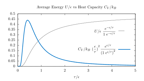
For a single particle with two states—energy 0 and energy $\epsilon$—in thermal contact with a reservoir at temperature $\tau$, the average energy $U$ and heat capacity $C_V$ are given by

\[ U ~=~ \epsilon\,\frac{e^{-\epsilon/\tau}}{1 + e^{-\epsilon/\tau}} \quad\text{and}\quad C_V ~=~ k_B\,\left(\frac{\epsilon}{\tau}\right)^2 \frac{e^{\epsilon/\tau}}{\left(1 + e^{\epsilon/\tau}\right)^2} \]

where $k_B \approx 1.38065 \times 10^{\text{$-$}23}$ J/K is the Boltzmann constant. The graph below shows both quantities as functions of $\tau/\epsilon$ (not $\epsilon/\tau$, as you might expect). See Exercise 9.

thermalex

Exercises

For Exercises 1-8 sketch the graph of the given function. Find all local maxima and minima, inflection points, where the function is increasing or decreasing, where the function is concave up or concave down, and indicate any asymptotes.

$f(x) ~=~ x^3 - 3x\vphantom{;e^{-x^2}}$
$f(x) ~=~ x^3 - 3x^2 + 1\vphantom{;e^{-x^2}}$
$f(x) ~=~ xe^{-x}\vphantom{;e^{-x^2}}$
$f(x) ~=~ x^2 \;e^{-x^2}$

4
$f(x) ~=~ \dfrac{1}{1 ~+~ x^2}\vphantom{\dfrac{e^{-x} ~-~ e^{-2x}}{2}}$
$f(x) ~=~ \dfrac{x^2}{(x - 1)^2}\vphantom{\dfrac{e^{-x} ~-~ e^{-2x}}{2}}$
$f(x) ~=~ \dfrac{e^{-x} ~-~ e^{-2x}}{2}$
$f(x) ~=~ e^{-x}\;\sin\,x\vphantom{\dfrac{e^{-x} ~-~ e^{-2x}}{2}}$
Write $U/\epsilon$ and $C_V/k_B$ from Example 4.13 as functions of $x=\tau/\epsilon$. You do not need to sketch the graphs.
Show that the function $D(r) = \frac{4}{a_0^3}\,r^2 e^{-2r/a_0}$ from Example 4.12 has a local maximum at $r=a_0$ and inflection points at $r = \left(1 \pm \frac{1}{\sqrt{2}}\right)\,a_0$.
Sketch the graph of Kratzer’s molecular potential $V(r) = -2D\,\left(\frac{a}{r} - \frac{1}{2} \frac{a^2}{r^2}\right)$ as a function of $x=\frac{r}{a}$, with $a > 0$ and $D > 0$ as constants.
Sketch the graph of $f(K) = \frac{2N\sqrt{K}\,e^{-\frac{K}{kT}}}{\sqrt{\pi}\,(kT)^{3/2}}$ as a function of $x=\frac{K}{kT}$, with $N$, $k$ and $T$ as positive constants.
Prove part (b) of the Concavity Theorem.

For a proof, see pp.10-11 in Koo, D., Elements of Optimization, New York: Springer-Verlag, 1977. ↩

\(x\) values	\(3\,(x-1)\)	\((x-3)\)	\(f'(x)\)	direction
\(x < 1\)	\(-\)	\(-\)	\(+\)	\(f\) is increasing
\(1 < x < 3\)	\(+\)	\(-\)	\(-\)	\(f\) is decreasing
\(x > 3\)	\(+\)	\(+\)	\(+\)	\(f\) is increasing