1.3 The Derivative: Infinitesimal Approach

Traditionally a function \(f\) of a variable \(x\) is written as \(y=f(x)\). The dependent variable \(y\) is considered a function of the independent variable \(x\). This allows taking the derivative of \(y\) with respect to \(x\), i.e. the derivative of \(y\) as a function of \(x\), denoted by \(\dydx\). This is simply a different way of writing \(f'(x)\), and is just one of many ways of denoting the derivative:

The notation \(\dydx\) appears to denote a fraction: a quantity \(\dy\) divided by a quantity \(\dx\). It turns out that the derivative really can be thought of in that way, as a ratio of infinitesimals. In fact, this was the way in which derivatives were used by the founders of calculus—Newton and, in particular, Leibniz.^[1] Even today, this is often the way in which derivatives are thought of and used in fields outside of mathematics, such as physics, engineering, and chemistry, perhaps due to its more intuitive nature.

The concept of infinitesimals used here is based on the nilsquare infinitesimal approach developed by J.L. Bell^[2], namely:

The above definition says that infinitesimals are numbers which are closer to 0 than any positive or negative number without being zero themselves, and raising them to powers greater than or equal to 2 makes them 0. So infinitesimals are not real numbers.^[3] This is not a problem, since calculus deals with other numbers, such as infinity, which are not real. An infinitesimal can be thought of as an infinitely small number arbitrarily close to 0 but not 0. This might seem like a strange notion, but it really is not all that different from the limit notion where, say, you let \(\Delta x\) approach 0 but not necessarily let it equal 0.^[4]

As for the square of a nonzero infinitesimal being 0, think of how a calculator handles the squares of small numbers. For example, most calculators can display \(10^{-8}\) as 0.00000001, and will even let you add 1 to that to get 1.00000001. But when you square \(10^{-8}\) and add 1 to it, most calculators will display the sum as simply 1. The calculator treats the square of \(10^{-8}\), namely \(10^{-16}\), as a number so small compared to 1 that it is effectively zero.^[5]

Notice a major difference between 0 and an infinitesimal \(\delta\): \(2 \cdot 0\) and \(0\) are the same, but \(2\,\delta\) and \(\delta\) are distinct. This holds for any nonzero constant multiple, not just the number 2.

The derivative \(\dydx\) of a function \(y=f(x)\) can now be defined in terms of infinitesimals:

The basic idea is that \(\dx\) is an infinitesimally small change in the variable \(x\), producing an infinitesimally small change \(\dy\) in the value of \(y=f(x)\).

You might have noticed that the above example did not involve limits, and that the derivative \(2x\) represents a real number (i.e. no infinitesimals appear in the final answer); this will always be the case. Infinitesimals possess another useful property:

In other words, at the infinitesimal level differentiable curves are straight. The idea behind this is simple. At various points on a nonstraight differentiable curve \(y=f(x)\) the distances along the curve between the points are not quite the same as the lengths of the line segments joining the points. For example, in Figure 1.3.1 the distance \(s\) measured along the curve from the point \(A\) to the point \(B\) is not the same as the length of the line segment \(\overline{AB}\) joining \(A\) to \(B\).

However, as the points \(A\) and \(B\) get closer to each other, the difference between that part of the curve joining \(A\) to \(B\) and the line segment \(\overline{AB}\) becomes less noticeable. That is, the curve is almost linear when \(A\) and \(B\) are close. The Microstraightness Property simply goes one step further and says that the curve actually is linear when the distance \(s\) between the points is infinitesimal (so that \(s\) equals the length of \(\overline{AB}\) at the infinitesimal level).

At first this might seem nonsensical. After all, how could any nonstraight part of a curve be straight? You have to remember that an infinitesimal is an abstraction—it does not exist physically. A curve \(y=f(x)\) is also an abstraction, which exists in a purely mathematical sense, so its geometric properties at the “normal” scale do not have to match those at the infinitesimal scale (which can be defined in any way, provided the properties at that scale are consistent).

[r] This abstraction finally reveals what an instantaneous rate of change is: the average rate of change over an infinitesimal interval. Moving an infinitesimal amount \(\dx\) away from a value \(x\) produces an infinitesimal change \(\dy\) in a differentiable function \(y=f(x)\). The average rate of change of \(y=f(x)\) over the infinitesimal interval \(\ival{x}{x+\dx}\) is thus \(\dydx\), i.e. the slope—rise over run—of the straight line segment represented by the curve \(y=f(x)\) over that interval, as in the figure on the right.^[6] The Microstraightness Property can be extended to smooth curves—that is, curves without sharp edges or cusps. For example, circles and ellipses are smooth, but polygons are not.

The properties of infinitesimals can be applied to determine the derivatives of the sine and cosine functions. Consider a circle of radius 1 with center \(O\) and points \(A\) and \(B\) on the circle such that the line segment \(\overline{AB}\) is a diameter. Let \(C\) be a point on the circle such that the angle \(\angle\,BAC\) has an infinitesimal measure \(\dx\) (in radians) as in Figure 1.3.2(a).

By Thales’ Theorem from elementary geometry, the angle \(\angle\,ACB\) is a right angle. Thus:

Figure 1.3.2(b) shows that \(\angle\,OAC + \angle\,OCA + \angle\,AOC = \pi\). Thus, \(1=OC=OA \Rightarrow \angle\,OCA = \angle\,OAC = \dx \Rightarrow \angle\,AOC = \pi-\dx-\dx = \pi-2\dx \Rightarrow \angle\,BOC = 2\dx\). By the arc length formula from trigonometry, the length \(s\) of the arc \(\wideparen{BC}\) along the circle from \(B\) to \(C\) is the radius times the central angle \(\angle\,BOC\): \(s = \wideparen{BC} = 1 \cdot 2\dx = 2\dx\). But by Microstraightness, \(\wideparen{BC} = BC\), and thus:

Since \(\dx\) is an infinitesimal, \(( \dx )^2 = 0\). So since \(\sin^2 \,\dx + \cos^2 \,\dx = 1\), then:

The derivative of \(y=\sin\,x\) is then:

A similar argument (left as an exercise) using the cosine addition formula shows:

One of the intermediate results proved here bears closer examination. Namely, \(\sin\,\dx = \dx\) for an infinitesimal angle \(\dx\) measured in radians. At first, it might seem that this cannot be true. After all, an infinitesimal \(\dx\) is thought of as being infinitely close to 0, and \(\sin\,0 = 0\), so you might expect that \(\sin\,\dx = 0\). But this is not the case. The formula \(\sin\,\dx = \dx\) says that in an infinitesimal interval around 0, the function \(y=\sin\,x\) is identical to the line \(y=x\) (not the line \(y=0\)). This, in turn, suggests that for real-valued \(x\) close to \(0\), \(\sin\,x \approx x\).

This indeed turns out to be the case. The free graphing software Gnuplot^[7] can display the graphs of \(y=\sin\,x\) and \(y=x\). Figure 1.3.3(a) below shows how those graphs compare over the interval \(\ival{-\pi}{\pi}\). Outside the interval \(\ival{-1}{1}\) there is a noticeable difference.

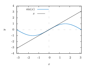
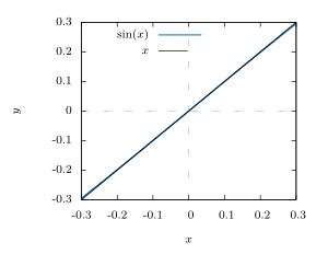
Figure 1.3.3(b) shows that there is virtually no difference in the graphs even over the non-infinitesimal interval \(\ival{-0.3}{0.3}\). So \(\sin\,x \approx x\) is a good approximation when \(x\) is close to 0, that is, when \(\abs{x} \ll 1\) (the symbol \(\ll\) means “much less than”). This approximation is used in many applications in engineering and physics when the angle \(x\) is assumed to be small.

Notice something else suggested by the relation \(\sin\,\dx = \dx\): there is a fundamental difference at the infinitesimal level between a line of slope 1 (\(y=x\)) and a line of slope 0 (\(y=0\)). In a real interval \((-a,a)\) around \(x=0\) the difference between the two lines can be made as small as desired by choosing \(a>0\) small enough. But in an infinitesimal interval \((-\delta,\delta)\) around \(x=0\) there is unbridgeable gulf between the two lines. This is the crucial difference in \(\sin\,\dx\) being equal to \(\dx\) rather than 0.

Notice also that the value of a function at an infinitesimal may itself be an infinitesimal (e.g. \(\sin\,\dx = \dx\)) or a real number (e.g. \(\cos\,\dx = 1\)).

For a differentiable function \(f(x)\), \(\dfdx = f'(x)\) and so multiplying both sides by \(\dx\) yields the important relation:

Note that both sides of the above equation are infinitesimals for each value of \(x\) in the domain of \(f'\), since \(f'(x)\) would then be a real number.

The notion of an infinitesimal was fairly radical at the time (and still is). Some mathematicians embraced it, e.g. the outstanding Swiss mathematician Leonhard Euler (1707-1783), who produced a large amount of work using infinitesimals. But it was too radical for many mathematicians (and philosophers^[8]), enough so that by the 19^th century some mathematicians (notably Augustin Cauchy and Karl Weierstrass) felt the need to put calculus on what they considered a more “rigorous” footing, based on limits.^[9] Yet it was precisely the notion of an infinitesimal which lent calculus its modern character, by showing the power and usefulness of such an abstraction (especially one that did not obey the rules of classical mathematics).