So far in this chapter, we’ve considered initial value problems for the constant coefficient equation
where \(f\) is continuous or piecewise continuous on \([0,\infty)\). In this section we consider initial value problems where \(f\) represents a force that’s very large for a short time and zero otherwise. We say that such forces are impulsive. Impulsive forces occur, for example, when two objects collide. Since it isn’t feasible to represent such forces as continuous or piecewise continuous functions, we must construct a different mathematical model to deal with them.
If \(f\) is an integrable function and \(f(t)=0\) for \(t\) outside of the interval \([t_0,t_0+h]\), then \(\int_{t_0}^{t_0+h} f(t)\,dt\) is called the total impulse of \(f\). We’re interested in the idealized situation where \(h\) is so small that the total impulse can be assumed to be applied instantaneously at \(t=t_0\). We say in this case that \(f\) is an impulse function. In particular, we denote by \(\delta(t-t_0)\) the impulse function with total impulse equal to one, applied at \(t=t_0\). (The impulse function \(\delta(t)\) obtained by setting \(t_0=0\) is the Dirac \(\delta\) function.) It must be understood, however, that \(\delta(t-t_0)\) isn’t a function in the standard sense, since our “definition” implies that \(\delta(t-t_0)=0\) if \(t\ne t_0\), while
From calculus we know that no function can have these properties; nevertheless, there’s a branch of mathematics known as the theory of distributions where the definition can be made rigorous. Since the theory of distributions is beyond the scope of this book, we’ll take an intuitive approach to impulse functions.
Our first task is to define what we mean by the solution of the initial value problem
where \(t_0\) is a fixed nonnegative number. The next theorem will motivate our definition.
Theorem 8.7.1
Suppose \(t_0\ge0.\) For each positive number \(h,\) let \(y_h\) be the solution of the initial value problem
where
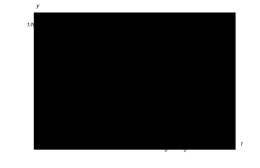
so \(f_h\) has unit total impulse equal to the area of the shaded rectangle in Figure \(\ref{figure:8.7.1}\). Then
where
Proof Taking Laplace transforms in (8.7.1) yields
so
The convolution theorem implies that
Therefore, (8.7.2) implies that
Since \(y_h(t)=0\) for all \(h\) if \(0\le t\le t_0\), it follows that
We’ll now show that
Suppose \(t\) is fixed and \(t>t_0\). From (8.7.4),
Since
we can write
From this and (8.7.7),
Therefore
Now let \(M_h\) be the maximum value of \(|w(t-\tau)-w(t-t_0)|\) as \(\tau\) varies over the interval \([t_0,t_0+h]\). (Remember that \(t\) and \(t_0\) are fixed.) Then (8.7.8) and (8.7.9) imply that
But \(\lim_{h\to0+}M_h=0\), since \(w\) is continuous. Therefore (8.7.10) implies (8.7.6). This and (8.7.5) imply (8.7.3). ∎
Theorem 8.7.1 motivates the next definition.
Definition 8.7.2
If \(t_0>0\), then the solution of the initial value problem
is defined to be
where
In physical applications where the input \(f\) and the output \(y\) of a device are related by the differential equation
\(w\) is called the impulse response of the device. Note that \(w\) is the solution of the initial value problem
as can be seen by using the Laplace transform to solve this problem. (Verify.) On the other hand, we can solve (8.7.12) by the methods of Section 5.2 and show that \(w\) is defined on \((-\infty,\infty)\) by
depending upon whether the polynomial \(p(r)=ar^2+br+c\) has distinct real zeros \(r_1\) and \(r_2\), a repeated zero \(r_1\), or complex conjugate zeros \(\lambda\pm i\omega\). (In most physical applications, the zeros of the characteristic polynomial have negative real parts, so \(\lim_{t\to\infty}w(t)=0\).) This means that \(y=u(t-t_0)w(t-t_0)\) is defined on \((-\infty,\infty)\) and has the following properties:
and
(remember that \(y'_-(t_0)\) and \(y'_+(t_0)\) are derivatives from the right and left, respectively) and \(y'(t_0)\) does not exist. Thus, even though we defined \(y=u(t-t_0)w(t-t_0)\) to be the solution of (8.7.11), this function doesn’t satisfy the differential equation in (8.7.11) at \(t_0\), since it isn’t differentiable there; in fact (8.7.14) indicates that an impulse causes a jump discontinuity in velocity. (To see that this is reasonable, think of what happens when you hit a ball with a bat.) This means that the initial value problem (8.7.11) doesn’t make sense if \(t_0=0\), since \(y'(0)\) doesn’t exist in this case. However \(y=u(t)w(t)\) can be defined to be the solution of the modified initial value problem
where the condition on the derivative at \(t=0\) has been replaced by a condition on the derivative from the left.
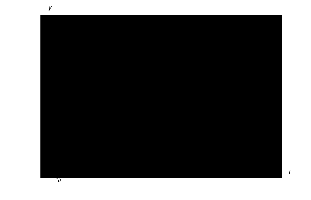
Figure 8.7.2 illustrates Theorem 8.7.1 for the case where the impulse response \(w\) is the first expression in (8.7.13) and \(r_1\) and \(r_2\) are distinct and both negative. The solid curve in the figure is the graph of \(w\). The dashed curves are solutions of (8.7.1) for various values of \(h\). As \(h\) decreases the graph of \(y_h\) moves to the left toward the graph of \(w\).
Example 8.7.1
Find the solution of the initial value problem
where \(t_0>0\). Then interpret the solution for the case where \(t_0=0\).
Solution Here
so Definition 8.7.2 yields
as the solution of (8.7.15) if \(t_0>0\). If \(t_0=0\), then (8.7.15) doesn’t have a solution; however, \(y=u(t)te^{-t}\) (which we would usually write simply as \(y=te^{-t}\)) is the solution of the modified initial value problem
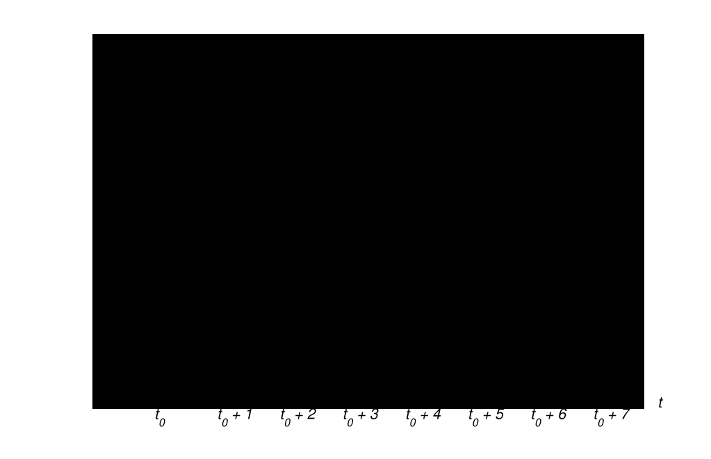
The graph of \(y=u(t-t_0)(t-t_0)e^{-(t-t_0)}\) is shown in Figure 8.7.3 ∎
Definition 8.7.2 and the principle of superposition motivate the next definition.
Definition 8.7.3
Suppose \(\alpha\) is a nonzero constant and \(f\) is piecewise continuous on \([0,\infty)\). If \(t_0>0\), then the solution of the initial value problem
is defined to be
where \(\hat y\) is the solution of
This definition also applies if \(t_0=0\), provided that the initial condition \(y'(0)=k_1\) is replaced by \(y_-'(0)=k_1\).
Example 8.7.2
Solve the initial value problem
Solution We leave it to you to show that the solution of
is
Since
the solution of (8.7.16) is
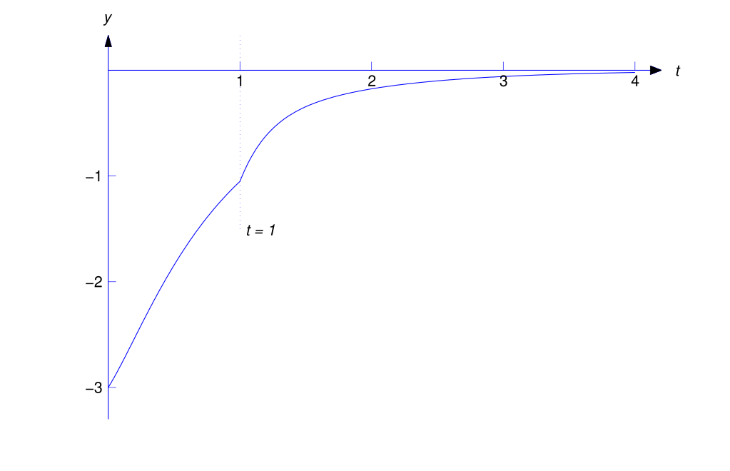
(Figure 8.7.4)∎.
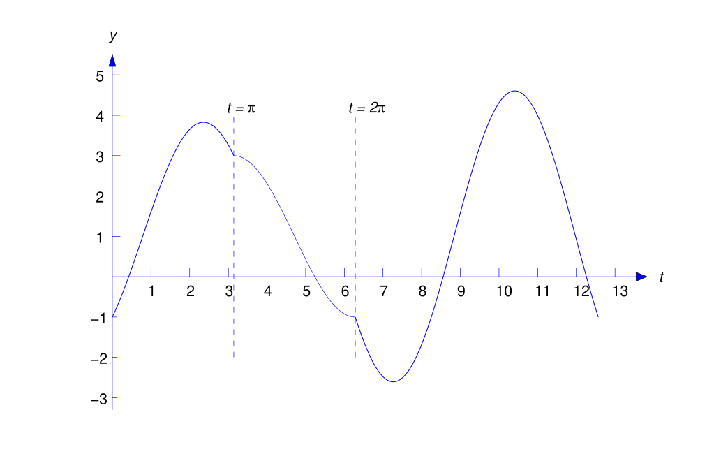
Definition 8.7.3 can be extended in the obvious way to cover the case where the forcing function contains more than one impulse.
Example 8.7.3
Solve the initial value problem
Solution We leave it to you to show that
is the solution of
Since
the solution of (8.7.18) is
or
(Figure 8.7.5).
8.7 Exercises
In Exercises 1–20 solve the initial value problem. Where indicated by C/G , graph the solution.
-
\(y''+3y'+2y=6e^{2t}+2\delta(t-1), \quad y(0)=2,\quad y'(0)=-6\)
Show answer
\(y=\dst{\frac{1}{2}e^{2t}-4e^{-t}+\frac{11}{2}e^{-2t}+2u(t-1)(e^{-(t-1)}-e^{-2(t-1)})}\)
-
C/G \(y''+y'-2y=-10e^{-t}+5\delta(t-1), \quad y(0)=7,\quad y'(0)=-9\)
Show answer
\(\dst{y=2e^{-2t}+5e^{-t}+\frac{5}{3}u(t-1)(e^{(t-1)}-e^{-2(t-1)})}\)
-
\(y''-4y=2e^{-t}+5\delta(t-1), \quad y(0)=-1,\quad y'(0)=2\)
Show answer
\(\dst{y=\frac{1}{6}e^{2t}-\frac{2}{3}e^{-t}-\frac{1}{2}e^{-2t}+\frac{5}{2}u(t-1)\sinh2(t-1)}\)
-
C/G \(y''+y=\sin3t+2\delta(t-\pi/2), \quad y(0)=1,\quad y'(0)=-1\)
Show answer
\(\dst{y=\frac{1}{8}(8\cos t-5\sin t-\sin3t)-2u(t-\pi/2)\cos t}\)
-
\(y''+4y=4+\delta(t-3\pi), \quad y(0)=0,\quad y'(0)=1\)
Show answer
\(\dst{y=1-\cos2t+\frac{1}{2}\sin2t+\frac{1}{2}u(t-3\pi)\sin2t}\)
-
\(y''-y=8+2\delta(t-2), \quad y(0)=-1,\quad y'(0)=1\)
Show answer
\(\dst{y=4e^{t}+3e^{-t}-8+2u(t-2)\sinh(t-2)}\)
-
\(y''+y'=e^t+3\delta(t-6), \quad y(0)=-1,\quad y'(0)=4\)
Show answer
\(\dst{y=\frac{1}{2}e^{t}-\frac{7}{2}e^{-t}+2+3u(t-6)(1-e^{-(t-6)})}\)
-
\(y''+4y=8e^{2t}+\delta(t-\pi/2), \quad y(0)=8,\quad y'(0)=0\)
Show answer
\(\dst{y=e^{2t}+7\cos 2t-\sin2t-\frac{1}{2}u(t-\pi/2)\sin 2t}\)
-
C/G \(y''+3y'+2y=1+\delta(t-1), \quad y(0)=1,\quad y'(0)=-1\)
Show answer
\(\dst{y=\frac{1}{2}(1+e^{-2t})+u(t-1)(e^{-(t-1)}-e^{-2(t-1)})}\)
-
\(y''+2y'+y=e^t+2\delta(t-2), \quad y(0)=-1,\quad y'(0)=2\)
Show answer
\(\dst{y=\frac{1}{4}e^{t}+\frac{1}{4}e^{-t}(2t-5)+2u(t-2)(t-2)e^{-(t-2)}}\)
-
C/G \(y''+4y=\sin t+\delta(t-\pi/2), \quad y(0)=0,\quad y'(0)=2\)
Show answer
\(\dst{y=\frac{1}{6}(2\sin t+5\sin 2t)-\frac{1}{2}u(t-\pi/2)\sin2t}\)
-
\(y''+2y'+2y=\delta(t-\pi)-3\delta(t-2\pi), \quad y(0)=-1,\quad y'(0)=2\)
Show answer
\(\dst{y=e^{-t}(\sin t-\cos t)-e^{-(t-\pi)}\sin t-3u(t-2\pi)e^{-(t-2\pi)}\sin t}\)
-
\(y''+4y'+13y=\delta(t-\pi/6)+2\delta(t-\pi/3), \quad y(0)=1,\quad y'(0)=2\)
Show answer
\(\dst{y=e^{-2t}\left(\cos 3t+\frac{4}{3}\sin3t\right)-\frac{1}{3} u(t-\pi/6)e^{-2(t-\pi/6)}\cos3t-\frac{2}{3}u(t-\pi/3)e^{-2(t-\pi/3)}\sin3t}\)
-
\(2y''-3y'-2y=1+\delta(t-2), \quad y(0)=-1,\quad y'(0)=2\)
Show answer
\(\dst{y=\frac{7}{10}e^{2t}-\frac{6}{5}e^{-t/2}-\frac{1}{2}+\frac{1}{5}u(t-2)} (e^{2(t-2)}-e^{-(t-2)/2})\)
-
\(4y''-4y'+5y=4\sin t-4\cos t+\delta(t-\pi/2)-\delta(t-\pi), \quad y(0)=1,\quad y'(0)=1\)
Show answer
\(\dst{y=\frac{1}{17}(12\cos t+20\sin t)+\frac{1}{34}e^{t/2}(10\cos t-11\sin t) -u(t-\pi/2)e^{(2t-\pi)/4}\cos t}\)
\(+u(t-\pi)e^{(t-\pi)/2}\sin t\)
-
\(y''+y=\cos2t+2\delta(t-\pi/2)-3\delta(t-\pi), \quad y(0)=0,\quad y'(0)=-1\)
Show answer
\(\dst{y=\frac{1}{3}(\cos t-\cos2t-3\sin t)-2u(t-\pi/2)\cos t+3u(t-\pi)\sin t}\)
-
C/G \(y''-y=4e^{-t}-5\delta(t-1)+3\delta(t-2), \quad y(0)=0,\quad y'(0)=0\)
Show answer
\(\dst{y=e^{t}-e^{-t}(1+2t)-5u(t-1)\sinh(t-1)+3u(t-2)\sinh (t-2)}\)
-
\(y''+2y'+y=e^t-\delta(t-1)+2\delta(t-2), \quad y(0)=0,\quad y'(0)=-1\)
Show answer
\(\dst{y=\frac{1}{4}(e^{t}-e^{-t}(1+6t))-u(t-1)e^{-(t-1)}+2u(t-2)e^{-(t-2)})}\)
-
\(y''+y=f(t)+\delta(t-2\pi), \quad y(0)=0,\quad y'(0)=1\), and
\(f(t)=\dst{\left\{\begin{array}{cl} \sin2t,&0\le t<\pi,\\[5pt]0,&t\ge \pi.\end{array}\right.}\)
Show answer
\(\dst{y=\frac{5}{3}\sin t-\frac{1}{3}\sin2t+\frac{1}{3}u(t-\pi)(\sin2t+2\sin t) +u(t-2\pi)\sin t}\)
-
\(y''+4y=f(t)+\delta(t-\pi)-3\delta(t-3\pi/2), \quad y(0)=1,\quad y'(0)=-1\), and
\(f(t)=\dst{\left\{\begin{array}{cl}1,&0\le t<\pi/2,\\[5pt]2,&t\ge \pi/2\end{array}\right.}\)
Show answer
\(\dst{y=\frac{3}{4}\cos2t-\frac{1}{2}\sin2t+\frac{1}{4}+\frac{1}{4}u(t-\pi/2) (1+\cos2t)+\frac{1}{2}u(t-\pi)\sin2t+\frac{3}{2}u(t-3\pi/2)\sin 2t}\)
-
\(y''+y=\delta(t), \quad y(0)=1,\quad y_-'(0)=-2\)
Show answer
\(y=\cos t-\sin t\)
-
\(y''-4y=3\delta(t), \quad y(0)=-1,\quad y_-'(0)=7\)
Show answer
\(\dst{y=\frac{1}{4}(8e^{3t}-12e^{-2t})}\)
-
\(y''+3y'+2y=-5\delta(t), \quad y(0)=0,\quad y_-'(0)=0\)
Show answer
\(\dst{y=5(e^{-2t}-e^{-t})}\)
-
\(y''+4y'+4y=-\delta(t), \quad y(0)=1,\quad y_-'(0)=5\)
Show answer
\(y=e^{-2t}(1+6t)\)
-
\(4y''+4y'+y=3\delta(t), \quad y(0)=1,\quad y_-'(0)=-6\)
Show answer
\(\dst{y=\frac{1}{4}e^{-t/2}(4-19t)}\)
In Exercises 26-28, solve the initial value problem
where \(t_0>0\) and \(h>0\). Then find
and verify Theorem 8.7.1 by graphing \(w\) and \(y_h\) on the same axes, for small positive values of \(h\).
-
L \(y''+2y'+2y=f_h(t), \quad y(0)=0,\quad y'(0)=0\)
-
L \(y''+2y'+y=f_h(t), \quad y(0)=0,\quad y'(0)=0\)
-
L \(y''+3y'+2y=f_h(t), \quad y(0)=0,\quad y'(0)=0\)
-
Recall from Section 6.2 that the displacement of an object of mass \(m\) in a spring–mass system in free damped oscillation is
\[ my''+cy'+ky=0, \quad y(0)=y_0,\quad y'(0)=v_0, \]and that \(y\) can be written as
\[ y=Re^{-ct/2m}\cos(\omega_1t-\phi) \]if the motion is underdamped. Suppose \(y(\tau)=0\). Find the impulse that would have to be applied to the object at \(t=\tau\) to put it in equilibrium.
Show answer
\(\dst{y=(-1)^{k}m\omega_{1}Re^{-c\tau/2m}\delta(t-\tau)}\) if \(\omega_{1}\tau-\phi=(2k+1)\pi/2\) (\(k=\) integer)
-
Solve the initial value problem. Find a formula that does not involve step functions and represents \(y\) on each subinterval of \([0,\infty)\) on which the forcing function is zero.
(a) \(\dst{y''-y=\sum_{k=1}^\infty\delta(t-k), \quad y(0)=0,\quad y'(0)=1}\)
(b) \(\dst{y''+y=\sum_{k=1}^\infty\delta(t-2k\pi), \quad y(0)=0,\quad y'(0)=1}\)
(c) \(\dst{y''-3y'+2y=\sum_{k=1}^\infty\delta(t-k), \quad y(0)=0,\quad y'(0)=1}\)
(d) \(\dst{y''+y=\sum_{k=1}^\infty\delta(t-k\pi), \quad y(0)=0,\quad y'(0)=0}\)
Show answer
(a) \(\dst{y=\frac{(e^{m+1}-1)(e^{t-m}-e^{-t})}{2(e-1)}}\), \(m\le t<m+1\), (\(m=0\), \(1\), …)
(b) \(y=(m+1)\sin t\), \(2m\pi\le t<2(m+1)\pi\), (\(m=0\), \(1\), …)
(c) \(\dst{y=e^{2(t-m)}\frac{e^{2m+2}-1}{e^{2}-1}-e^{(t-m)}\frac{e^{m+1}-1}{e-1}}\), \(m\le t<m+1\) (\(m=0\), \(1\), …)
(d) \(y= \begin{cases} \quad\, 0,&\quad 2m\pi\le t<(2m+1)\pi,\\ -\sin t,& (2m+1)\pi\le t <(2m+2)\pi, \end{cases}\) (\(m=0\), \(1\),…)