6.3 The $RLC$ Circuit

In this section we consider the $RLC$ circuit, shown schematically in Figure 6.3.1. As we’ll see, the $RLC$ circuit is an electrical analog of a spring-mass system with damping.

Nothing happens while the switch is open (dashed line). When the switch is closed (solid line) we say that the circuit is closed. Differences in electrical potential in a closed circuit cause current to flow in the circuit. The battery or generator in Figure 6.3.1 creates a difference in electrical potential $E=E(t)$ between its two terminals, which we’ve marked arbitrarily as positive and negative. (We could just as well interchange the markings.) We’ll say that $E(t)>0$ if the potential at the positive terminal is greater than the potential at the negative terminal, $E(t)<0$ if the potential at the positive terminal is less than the potential at the negative terminal, and $E(t)=0$ if the potential is the same at the two terminals. We call $E$ the impressed voltage.

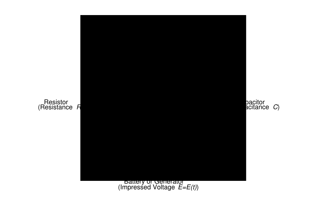
An RLC circuit — Figure 6.3.1. An $RLC$ circuit

At any time $t$, the same current flows in all points of the circuit. We denote current by $I=I(t)$. We say that $I(t)>0$ if the direction of flow is around the circuit from the positive terminal of the battery or generator back to the negative terminal, as indicated by the arrows in Figure 6.3.1 $I(t)<0$ if the flow is in the opposite direction, and $I(t)=0$ if no current flows at time $t$.

Differences in potential occur at the resistor, induction coil, and capacitor in Figure 6.3.1. Note that the two sides of each of these components are also identified as positive and negative. The voltage drop across each component is defined to be the potential on the positive side of the component minus the potential on the negative side. This terminology is somewhat misleading, since “drop” suggests a decrease even though changes in potential are signed quantities and therefore may be increases. Nevertheless, we’ll go along with tradition and call them voltage drops. The voltage drop across the resistor in Figure 6.3.1 is given by

\begin{equation} V_R=IR, \tag{6.3.1}\end{equation}

where $I$ is current and $R$ is a positive constant, the resistance of the resistor. The voltage drop across the induction coil is given by

\begin{equation} V_I=L{dI\over dt}=LI', \tag{6.3.2}\end{equation}

where $L$ is a positive constant, the inductance of the coil.

A capacitor stores electrical charge $Q=Q(t)$, which is related to the current in the circuit by the equation

\begin{equation} Q(t)=Q_0+\int_0^tI(\tau)\,d\tau, \tag{6.3.3}\end{equation}

where $Q_0$ is the charge on the capacitor at $t=0$. The voltage drop across a capacitor is given by

\begin{equation} V_C={Q\over C}, \tag{6.3.4}\end{equation}

where $C$ is a positive constant, the capacitance of the capacitor.

Table 6.3.1 names the units for the quantities that we’ve discussed. The units are defined so that

\begin{eqnarray*} 1\mbox{\,volt}&=&1\mbox{\,ampere}\cdot1\mbox{\,ohm} \\ &=&1\mbox{\,henry}\cdot1\,\mbox{ampere}/\mbox{second} \\ &=&1\mbox{\,coulomb}/\mbox{\,farad} \\[6pt] \arraytext{and} \\ 1\mbox{\,ampere}&=&1\mbox{\,coulomb}/\mbox{second}. \end{eqnarray*}

Table 6.3.1. Electrical Units

Symbol	Name	Unit
$E$	Impressed Voltage	volt
$I$	Current	ampere
$Q$	Charge	coulomb
$R$	Resistance	ohm
$L$	Inductance	henry
$C$	Capacitance	farad

According to Kirchoff’s law, the sum of the voltage drops in a closed $RLC$ circuit equals the impressed voltage. Therefore, from (6.3.1), (6.3.2), and (6.3.4),

\begin{equation} LI'+RI+{1\over C}Q=E(t). \tag{6.3.5}\end{equation}

This equation contains two unknowns, the current $I$ in the circuit and the charge $Q$ on the capacitor. However, (6.3.3) implies that $Q'=I$, so (6.3.5) can be converted into the second order equation

\begin{equation} LQ''+RQ'+{1\over C}Q=E(t) \tag{6.3.6}\end{equation}

in $Q$. To find the current flowing in an $RLC$ circuit, we solve (6.3.6) for $Q$ and then differentiate the solution to obtain $I$.

In Sections 6.1 and 6.2 we encountered the equation

\begin{equation} my''+cy'+ky=F(t) \tag{6.3.7}\end{equation}

in connection with spring-mass systems. Except for notation this equation is the same as (6.3.6). The correspondence between electrical and mechanical quantities connected with (6.3.6) and (6.3.7) is shown in Table 6.3.2.

Table 6.3.2. Electrical and Mechanical Units

Electrical	Mechanical
charge	$Q$	displacement	$y$
curent	$I$	velocity	$y'$
impressed voltage	$E(t)$	external force	$F(t)$
inductance	$L$	Mass	$m$
resistance	$R$	damping	$c$
1/capacitance	$1/C$	cpring constant	$k$

The equivalence between (6.3.6) and (6.3.7) is an example of how mathematics unifies fundamental similarities in diverse physical phenomena. Since we’ve already studied the properties of solutions of (6.3.7) in Sections 6.1 and 6.2, we can obtain results concerning solutions of (6.3.6) by simpling changing notation, according to Table 6.3.1.

Free Oscillations

We say that an $RLC$ circuit is in free oscillation if $E(t)=0$ for $t>0$, so that (6.3.6) becomes

\begin{equation} LQ''+RQ'+{1\over C}Q=0. \tag{6.3.8}\end{equation}

The characteristic equation of (6.3.8) is

\[ Lr^2+Rr+{1\over C}=0, \]

with roots

\begin{equation} r_1={-R-\sqrt{R^2-4L/C}\over2L}\mbox{\quad and \quad} r_2= {-R+\sqrt{R^2-4L/C}\over2L}. \tag{6.3.9}\end{equation}

There are three cases to consider, all analogous to the cases considered in Section 6.2 for free vibrations of a damped spring-mass system.

Case 1. The oscillation is underdamped if $R<\sqrt{4L/C}$. In this case, $r_1$ and $r_2$ in (6.3.9) are complex conjugates, which we write as

\[ r_1=-{R\over2L}+i\omega_1\mbox{\quad and \quad} r_2=-{R\over2L}-i\omega_1, \]

where

\[ \omega_1={\sqrt{4L/C-R^2}\over2L}. \]

The general solution of (6.3.8) is

\[ Q=e^{-Rt/2L}(c_1\cos\omega_1 t+c_2\sin\omega_1 t), \]

which we can write as

\begin{equation} Q=Ae^{-Rt/2L}\cos(\omega_1 t-\phi), \tag{6.3.10}\end{equation}

where

\[ A=\sqrt{c_1^2+c_2^2},\quad A\cos\phi=c_1,\mbox{\quad and \quad} A\sin\phi=c_2. \]

In the idealized case where $R=0$, the solution (6.3.10) reduces to

\[ Q=A\cos\left({t\over\sqrt{LC}}-\phi\right), \]

which is analogous to the simple harmonic motion of an undamped spring-mass system in free vibration.

Actual $RLC$ circuits are usually underdamped, so the case we’ve just considered is the most important. However, for completeness we’ll consider the other two possibilities.

Case 2. The oscillation is overdamped if $R>\sqrt{4L/C}$. In this case, the zeros $r_1$ and $r_2$ of the characteristic polynomial are real, with $r_1<r_2<0$ (see (6.3.9)), and the general solution of (6.3.8) is

\begin{equation} Q=c_1e^{r_1t}+c_2e^{r_2t}. \tag{6.3.11}\end{equation}

Case 3. The oscillation is critically damped if $R=\sqrt{4L/C}$. In this case, $r_1=r_2=-R/2L$ and the general solution of (6.3.8) is

\begin{equation} Q=e^{-Rt/2L}(c_1+c_2t). \tag{6.3.12}\end{equation}

If $R\ne0$, the exponentials in (6.3.10), (6.3.11), and (6.3.12) are negative, so the solution of any homogeneous initial value problem

\[ LQ''+RQ'+{1\over C}Q=0,\quad Q(0)=Q_0,\quad Q'(0)=I_0, \]

approaches zero exponentially as $t\to\infty$. Thus, all such solutions are transient, in the sense defined Section 6.2 in the discussion of forced vibrations of a spring-mass system with damping.

Example 6.3.1

At $t=0$ a current of 2 amperes flows in an $RLC$ circuit with resistance $R=40$ ohms, inductance $L=.2$ henrys, and capacitance $C=10^{-5}$ farads. Find the current flowing in the circuit at $t>0$ if the initial charge on the capacitor is 1 coulomb. Assume that $E(t)=0$ for $t>0$.

Solution The equation for the charge $Q$ is

\[ {1\over5}Q''+40Q'+10000Q=0, \]

\begin{equation} Q''+200Q'+50000Q=0. \tag{6.3.13}\end{equation}

Therefore we must solve the initial value problem

\begin{equation} Q''+200Q'+50000Q=0,\quad Q(0)=1,\quad Q'(0)=2. \tag{6.3.14}\end{equation}

The desired current is the derivative of the solution of this initial value problem.

The characteristic equation of (6.3.13) is

\[ r^2+200r+50000=0, \]

which has complex zeros $r=-100\pm200i$. Therefore the general solution of (6.3.13) is

\begin{equation} Q=e^{-100t}(c_1\cos200t+c_2\sin200t). \tag{6.3.15}\end{equation}

Differentiating this and collecting like terms yields

\begin{equation} Q'=-e^{-100t}\left[(100c_1-200c_2)\cos200t+ (100c_2+200c_1)\sin200t\right]. \tag{6.3.16}\end{equation}

To find the solution of the initial value problem (6.3.14), we set $t=0$ in (6.3.15) and (6.3.16) to obtain

\[ c_1=Q(0)=1\mbox{\quad and \quad} -100c_1+200c_2=Q'(0)=2; \]

therefore, $c_1=1$ and $c_2=51/100$, so

\[ Q=e^{-100t}\left(\cos200t+{51\over100}\sin200t\right) \]

is the solution of (6.3.14). Differentiating this yields

\[ I=e^{-100t}(2\cos200t-251\sin200t). \]

Forced Oscillations With Damping

An initial value problem for (6.3.6) has the form

\begin{equation} LQ''+RQ'+{1\over C}Q=E(t),\quad Q(0)=Q_0,\quad Q'(0)=I_0, \tag{6.3.17}\end{equation}

where $Q_0$ is the initial charge on the capacitor and $I_0$ is the initial current in the circuit. We’ve already seen that if $E\equiv0$ then all solutions of (6.3.17) are transient. If $E\not\equiv0$, we know that the solution of (6.3.17) has the form $Q=Q_c+Q_p$, where $Q_c$ satisfies the complementary equation, and approaches zero exponentially as $t\to\infty$ for any initial conditions , while $Q_p$ depends only on $E$ and is independent of the initial conditions. As in the case of forced oscillations of a spring-mass system with damping, we call $Q_p$ the steady state charge on the capacitor of the $RLC$ circuit. Since $I=Q'=Q_c'+Q_p'$ and $Q_c'$ also tends to zero exponentially as $t\to\infty$, we say that $I_c=Q'_c$ is the transient current and $I_p=Q_p'$ is the steady state current. In most applications we’re interested only in the steady state charge and current.

Example 6.3.2

Find the amplitude-phase form of the steady state current in the $RLC$ circuit in Figure 6.3.1 if the impressed voltage, provided by an alternating current generator, is $E(t)=E_0\cos\omega t$.

Solution We’ll first find the steady state charge on the capacitor as a particular solution of

\[ LQ''+RQ'+{1\over C}Q=E_0\cos\omega t. \]

To do, this we’ll simply reinterpret a result obtained in Section 6.2, where we found that the steady state solution of

\[ my''+cy'+ky=F_0\cos\omega t \]

\[ y_p={F_0\over\sqrt{(k-m\omega^2)^2+c^2\omega^2}} \cos(\omega t-\phi), \]

where

\[ \cos\phi={k-m\omega^2\over\sqrt {(k-m\omega^2)^2+c^2\omega^2}}\mbox{\quad and \quad} \sin\phi={c\omega\over\sqrt{(k-m\omega^2)^2+c^2\omega^2}}. \]

(See Equations (6.2.14) and (6.2.15).) By making the appropriate changes in the symbols (according to Table 2) yields the steady state charge

\[ Q_p={E_0\over\sqrt{(1/C-L\omega^2)^2+R^2\omega^2}}\cos(\omega t-\phi), \]

where

\[ \cos\phi={1/C-L\omega^2\over\sqrt{(1/C-L\omega^2)^2+R^2\omega^2}} \mbox{\quad and \quad} \sin\phi={R\omega\over\sqrt{(1/C-L\omega^2)^2+R^2\omega^2}}. \]

Therefore the steady state current in the circuit is

\[ I_p=Q_p'= -{\omega E_0\over\sqrt{(1/C-L\omega^2)^2+R^2\omega^2}}\sin(\omega t-\phi). \]

6.3 Exercises

In Exercises 1-5 find the current in the $RLC$ circuit, assuming that $E(t)=0$ for $t>0$.

$R=3$ ohms; $L=.1$ henrys; $C=.01$ farads; $Q_0=0$ coulombs; $I_0=2$ amperes.

Show answer

$I=e^{-15t}\dst{\left(2\cos5\sqrt{15}t- {6\over\sqrt{31}}\sin5\sqrt{31}t\right)}$
$R=2$ ohms; $L=.05$ henrys; $C=.01$ farads’; $Q_0=2$ coulombs; $I_0=-2$ amperes.

Show answer

$I=e^{-20t}(2\cos40t-101\sin40t)$
$R=2$ ohms; $L=.1$ henrys; $C=.01$ farads; $Q_0=2$ coulombs; $I_0=0$ amperes.

Show answer

$I=-\dst{200\over3}e^{-10t}\sin30t$
$R=6$ ohms; $L=.1$ henrys; $C=.004$ farads’; $Q_0=3$ coulombs; $I_0=-10$ amperes.

Show answer

$I=-10e^{-30t}(\cos40t+18\sin40t)$
$R=4$ ohms; $L=.05$ henrys; $C=.008$ farads; $Q_0=-1$ coulombs; $I_0=2$ amperes.

Show answer

$I=-e^{-40t}(2\cos30t-86\sin30t)$

In Exercises 6-10 find the steady state current in the circuit described by the equation.

$\dst{1\over10}Q''+3Q'+100Q=5\cos10t-5\sin10t$

Show answer

$I_p=\dst-{1\over3}(\cos10t+2\sin10t)$
$\dst{1\over20}Q''+2Q'+100Q=10\cos25t-5\sin25t$

Show answer

$I_p=\dst{20\over37}(\cos25t-6\sin25t)$
$\dst{1\over10}Q''+2Q'+100Q=3\cos50t-6\sin50t$

Show answer

$I_p= \dst{3\over13}(8\cos50t-\sin50t)$
$\dst{1\over10}Q''+6Q'+250Q=10\cos100t+30\sin100t$

Show answer

$I_p=\dst{20\over123}(17\sin100t-11\cos100t)$
$\dst{1\over20}Q''+4Q'+125Q=15\cos30t-30\sin30t$

Show answer

$I_p=-\dst{45\over52}(\cos30t+8\sin30t)$
Show that if $E(t)=U\cos\omega t+V\sin\omega t$ where $U$ and $V$ are constants then the steady state current in the $RLC$ circuit shown in Figure 6.3.1 is

\[ I_p={\omega^2RE(t)+(1/C-L\omega^2)E'(t)\over\Delta}, \]

where

\[ \Delta=(1/C-L\omega^2)^2+R^2\omega^2. \]
Find the amplitude of the steady state current $I_p$ in the $RLC$ circuit shown in Figure 6.3.1 if $E(t)=U\cos\omega t+V\sin\omega t$, where $U$ and $V$ are constants. Then find the value $\omega_0$ of $\omega$ maximizes the amplitude, and find the maximum amplitude.

Show answer

$\omega_0=1/\sqrt{LC}$ maximum amplitude $=\sqrt{U^2+V^2}/R$

In Exercises 13-17 plot the amplitude of the steady state current against $\omega$. Estimate the value of $\omega$ that maximizes the amplitude of the steady state current, and estimate this maximum amplitude. Hint: You can confirm your results by doing Exercise $\ref{exer:6.3.12}$.

L $\dst{1\over10}Q''+3Q'+100Q=U\cos\omega t+V\sin\omega t$
L $\dst{1\over20}Q''+2Q'+100Q=U\cos\omega t+V\sin\omega t$
L $\dst{1\over10}Q''+2Q'+100Q=U\cos\omega t+V\sin\omega t$
L $\dst{1\over10}Q''+6Q'+250Q=U\cos\omega t+V\sin\omega t$
L $\dst{1\over20}Q''+4Q'+125Q=U\cos\omega t+V\sin\omega t$

6.3 The \(RLC\) Circuit

Free Oscillations

Forced Oscillations With Damping

6.3 Exercises