13.2 Sturm-Liouville Problems

In this section we consider eigenvalue problems of the form

\begin{equation} P_{0}(x)y''+P_{1}(x)y'+P_{2}(x)y+ \lambda R(x)y=0,\quad B_{1}(y)=0,\quad B_{2}(y)=0, \tag{13.2.1}\end{equation}

where

\[ B_{1}(y)=\alpha y(a)+\beta y'(a) \text{\quad and\quad} B_{2}(y)=\rho y(b)+\delta y'(b). \]

As in Section 13.1, \(\alpha\), \(\beta\), \(\rho\), and \(\delta\) are real numbers, with

\[ \alpha^{2}+\beta^{2}>0\text{\; and\; \; } \rho^{2}+\delta^{2}>0, \]

\(P_{0}\), \(P_{1}\), \(P_{2}\), and \(R\) are continuous, and \(P_{0}\) and \(R\) are positive on \([a,b]\).

We say that \(\lambda\) is an eigenvalue of (13.2.1) if (13.2.1) has a nontrivial solution \(y\). In this case, \(y\) is an eigenfunction associated with \(\lambda\), or a \(\lambda\)-eigenfunction. Solving the eigenvalue problem means finding all eigenvalues and associated eigenfunctions of (13.2.1).

Example 13.2.1

Solve the eigenvalue problem

\begin{equation} y'+3y'+2y+\lambda y=0,\quad y(0)=0,\quad y(1)=0. \tag{13.2.2}\end{equation}

Solution The characteristic equation of (13.2.2) is

\[ r^{2}+3r+2+\lambda=0, \]

with zeros

\[ r_{1}=\frac{-3+\sqrt{1-4\lambda}}{2} \text{\quad and \quad } r_{2}=\frac{-3-\sqrt{1-4\lambda}}{2}. \]

If \(\lambda<1/4\) then \(r_{1}\) and \(r_{2}\) are real and distinct, so the general solution of the differential equation in (13.2.2) is

\[ y=c_{1}e^{r_{1}t}+c_{2}e^{r_{2}t}. \]

The boundary conditions require that

\begin{eqnarray*} c_{1}\phantom{e^{r_{1}}}+c_{2}\phantom{e^{r_{2}}}&=&0 \\ c_{1}e^{r_{1}}+c_{2}e^{r_{2}}&=&0. \end{eqnarray*}

Since the determinant of this system is \(e^{r_{2}}-e^{r_{1}}\ne0\), the system has only the trivial solution. Therefore \(\lambda\) isn’t an eigenvalue of (13.2.2).

If \(\lambda=1/4\) then \(r_{1}=r_{2}=-3/2\), so the general solution of (13.2.2) is

\[ y=e^{-3x/2}(c_{1}+c_{2}x). \]

The boundary condition \(y(0)=0\) requires that \(c_{1}=0\), so \(y=c_{2}xe^{-3x/2}\) and the boundary condition \(y(0)\) requires that \(c_{2}=0\). Therefore \(\lambda=1/4\) isn’t an eigenvalue of (13.2.2).

If \(\lambda>1/4\) then

\[ r_{1}=-\frac{3}{2}+i\omega \text{\quad and\quad } r_{2}=-\frac{3}{2}-i\omega, \]

with

\begin{equation} \omega =\frac{\sqrt{4\lambda-1}}{2} \text{\quad or, equivalently,\quad } \lambda=\frac{1+4\omega^{2}}{4}. \tag{13.2.3}\end{equation}

In this case the general solution of the differential equation in (13.2.2) is

\[ y=e^{-3x/2}(c_{1}\cos\omega x+c_{2}\sin\omega x). \]

The boundary condition \(y(0)=0\) requires that \(c_{1}=0\), so \(y=c_{2}e^{-3x/2}\sin\omega x\), which holds with \(c_{2}\ne0\) if and only if \(\omega=n\pi\), where \(n\) is an integer. We may assume that \(n\) is a positive integer. (Why?). From (13.2.3), the eigenvalues are \(\lambda_{n}=(1+4n^{2}\pi^{2})/4\), with associated eigenfunctions

\[ y_{n}=e^{-3x/2}\sin n\pi x,\quad n=1,2,3,\dots. \]

Example 13.2.2

Solve the eigenvalue problem

\begin{equation} x^{2}y''+xy'+\lambda y=0,\quad y(1)=0,\quad y(2)=0. \tag{13.2.4}\end{equation}

Solution If \(\lambda=0\), the differential equation in (13.2.4) reduces to \(x(xy')'=0\), so \(xy'=c_{1}\),

\[ y'=\frac{c_{1}}{x}, \text{\quad and\quad} y=c_{1}\ln x+c_{2}. \]

The boundary condition \(y(1)=0\) requires that \(c_{2}=0\), so \(y=c_{1}\ln x\). The boundary condition \(y(2)=0\) requires that \(c_{1}\ln2=0\), so \(c_{1}=0\). Therefore zero isn’t an eigenvalue of (13.2.4).

If \(\lambda<0\), we write \(\lambda=-k^{2}\) with \(k>0\), so (13.2.4) becomes

\[ x^{2}y''+xy'-k^{2}y=0, \]

an Euler equation (Section 7.4) with indicial equation

\[ r^{2}-k^{2}=(r-k)(r+k)=0. \]

Therefore

\[ y=c_{1}x^{k}+c_{2}x^{-k}. \]

The boundary conditions require that

\begin{eqnarray*} \phantom{2^{k}}c_{1}+\phantom{2^{-k}}c_{2}&=&0 \\ 2^{k}c_{1}+2^{-k}c_{2}&=&0. \end{eqnarray*}

Since the determinant of this system is \(2^{-k}-2^{k}\ne0\), \(c_{1}=c_{2}=0\). Therefore (13.2.4) has no negative eigenvalues.

If \(\lambda>0\) we write \(\lambda=k^{2}\) with \(k>0\). Then (13.2.4) becomes

\[ x^{2}y''+xy' +k^{2}y=0, \]

an Euler equation with indicial equation

\[ r^{2}+k^{2}=(r-ik)(r+ik)=0, \]

\[ y=c_{1}\cos(k\ln x)+c_{2}\sin(k\ln x). \]

The boundary condition \(y(1)=0\) requires that \(c_{1}=0\). Therefore \(y=c_{2}\sin(k\ln x)\). This holds with \(c_{2}\ne0\) if and only if \(k=n\pi/\ln 2\), where \(n\) is a positive integer. Hence, the eigenvalues of (13.2.4) are \(\lambda_{n}=(n\pi/\ln2)^{2}\), with associated eigenfunctions

\[ y_{n}=\sin\left(\frac{n\pi}{\ln2}\ln x\right),\quad n=1,2,3,\dots. \]

For theoretical purposes, it’s useful to rewrite the differential equation in (13.2.1) in a different form, provided by the next theorem.

Theorem 13.2.1

If \(P_{0},\) \(P_{1},\) \(P_{2},\) and \(R\) are continuous and \(P_{0}\) and \(R\) are positive on a closed interval \([a,b],\) then the equation

\begin{equation} P_{0}(x)y''+P_{1}(x)y'+P_{2}(x)y+\lambda R(x)y=0 \tag{13.2.5}\end{equation}

can be rewritten as

\begin{equation} (p(x)y')'+q(x)y+\lambda r(x)y=0, \tag{13.2.6}\end{equation}

where \(p\), \(p'\), \(q\) and \(r\) are continuous and \(p\) and \(r\) are positive on \([a,b].\)

Proof We begin by rewriting (13.2.5) as

\begin{equation} y''+u(x)y'+v(x)y+\lambda R_{1}(x)y=0, \tag{13.2.7}\end{equation}

with \(u=P_{1}/P_{0}\), \(v=P_{2}/P_{0}\), and \(R_{1}=R/P_{0}\). (Note that \(R_{1}\) is positive on \([a,b]\).) Now let \(p(x)=e^{U(x)}\), where \(U\) is any antiderivative of \(u\). Then \(p\) is positive on \([a,b]\) and, since \(U'=u\),

\begin{equation} p'(x)=p(x)u(x) \tag{13.2.8}\end{equation}

is continuous on \([a,b]\). Multiplying (13.2.7) by \(p(x)\) yields

\begin{equation} p(x)y''+p(x)u(x)y'+p(x)v(x)y+\lambda p(x)R_{1}(x)y=0. \tag{13.2.9}\end{equation}

Since \(p\) is positive on \([a,b]\), this equation has the same solutions as (13.2.5). From (13.2.8),

\[ (p(x)y')'=p(x)y''+p'(x)y'=p(x)y''+p(x)u(x)y', \]

so (13.2.9) can be rewritten as in (13.2.6), with \(q(x)=p(x)v(x)\) and \(r(x)=p(x)R_{1}(x)\). This completes the proof.

It is to be understood throughout the rest of this section that \(p\), \(q\), and \(r\) have the properties stated in Theorem 13.2.1. Moreover, whenever we write \(Ly\) in a general statement, we mean

\[ Ly=(p(x)y')'+q(x)y. \]

The differential equation (13.2.6) is called a Sturm– Liouville equation, and the eigenvalue problem

\begin{equation} (p(x)y')'+q(x)y+\lambda r(x)y=0,\quad B_{1}(y)=0,\quad B_{2}(y)=0, \tag{13.2.10}\end{equation}

which is equivalent to (13.2.1), is called a Sturm-Liouville problem.

Example 13.2.3

Rewrite the eigenvalue problem

\begin{equation} y''+3y'+(2+\lambda)y=0,\quad y(0)=0,\quad y(1)=0 \tag{13.2.11}\end{equation}

of Example 13.2.1 as a Sturm-Liouville problem.

Solution Comparing (13.2.11) to (13.2.7) shows that \(u(x)=3\), so we take \(U(x)=3x\) and \(p(x)=e^{3x}\). Multiplying the differential equation in (13.2.11) by \(e^{3x}\) yields

\[ e^{3x}(y''+3y')+2e^{3x}y+\lambda e^{3x}y=0. \]

Since

\[ e^{3x}(y''+3y')=(e^{3x}y')', \]

(13.2.11) is equivalent to the Sturm–Liouville problem

\begin{equation} (e^{3x}y')'+2e^{3x}y+\lambda e^{3x}y=0,\quad y(0)=0,\quad y(1)=0. \tag{13.2.12}\end{equation}

Example 13.2.4

Rewrite the eigenvalue problem

\begin{equation} x^{2}y''+xy'+\lambda y=0,\quad y(1)=0,\quad y(2)=0 \tag{13.2.13}\end{equation}

of Example 13.2.2 as a Sturm-Liouville problem.

Solution Dividing the differential equation in (13.2.13) by \(x^{2}\) yields

\[ y''+\frac{1}{x}y'+\frac{\lambda}{x^{2}}y=0. \]

Comparing this to (13.2.7) shows that \(u(x)=1/x\), so we take \(U(x)=\ln x\) and \(p(x)=e^{\ln x}=x\). Multiplying the differntial equation by \(x\) yields

\[ xy''+y'+\frac{\lambda}{x}y=0. \]

Since

\[ xy''+y'=(xy')', \]

(13.2.13) is equivalent to the Sturm–Liouville problem

\begin{equation} (xy')'+\frac{\lambda}{x}y=0,\quad y(1)=0,\quad y(2)=0. \tag{13.2.14}\end{equation}

∎

Problems 1–4 of Section 11.1 are Sturm–Liouville problems. (Problem 5 isn’t , although some authors use a definition of Sturm-Liouville problem that does include it.) We were able to find the eigenvalues of Problems 1-4 explicitly because in each problem the coefficients in the boundary conditions satisfy \(\alpha\beta=0\) and \(\rho\delta=0\); that is, each boundary condition involves either \(y\) or \(y'\), but not both. If this isn’t true then the eigenvalues can’t in general be expressed exactly by simple formulas; rather, approximate values must be obtained by numerical solution of equations derived by requiring the determinants of certain \(2\times 2\) systems of homogeneous equations to be zero. To apply the numerical methods effectively, graphical methods must be used to determine approximate locations of the zeros of these determinants. Then the zeros can be computed accurately by numerical methods.

Example 13.2.5

Solve the Sturm–Liouville problem

\begin{equation} y''+\lambda y=0, \quad y(0)+y'(0)=0,\quad y(1)+3y'(1)=0. \tag{13.2.15}\end{equation}

Solution If \(\lambda=0\), the differential equation in (13.2.15) reduces to \(y''=0\), with general solution \(y=c_{1}+c_{2}x\). The boundary conditions require that

\begin{eqnarray*} c_{1}+\phantom{4}c_{2}&=&0 \\ c_{1}+4c_{2}&=&0, \end{eqnarray*}

so \(c_{1}=c_{2}=0\). Therefore zero isn’t an eigenvalue of (13.2.15).

If \(\lambda<0\), we write \(\lambda=-k^{2}\) where \(k>0\), and the differential equation in (13.2.15) becomes \(y''-k^{2}y=0\), with general solution

\begin{equation} y=c_{1}\cosh kx+c_{2}\sinh kx, \tag{13.2.16}\end{equation}

\[ y'=k(c_{1}\sinh kx+c_{2}\cosh kx). \]

The boundary conditions require that

\begin{equation} \begin{gathered} c_{1}+kc_{2}=0\\ (\cosh k+3k\sinh k)c_{1}+(\sinh k+3k\cosh k)c_{2}=0. \end{gathered} \tag{13.2.17}\end{equation}

The determinant of this system is

\begin{eqnarray*} D_{N}(k)&=& \left|\begin{array}{cccccc} 1&k\\ \cosh k+3k\sinh k&\sinh k+3k \cosh k \end{array}\right| \\ &=& (1-3k^{2})\sinh k+2k \cosh k. \end{eqnarray*}

Therefore the system (13.2.17) has a nontrivial solution if and only if \(D_{N}(k)=0\) or, equivalently,

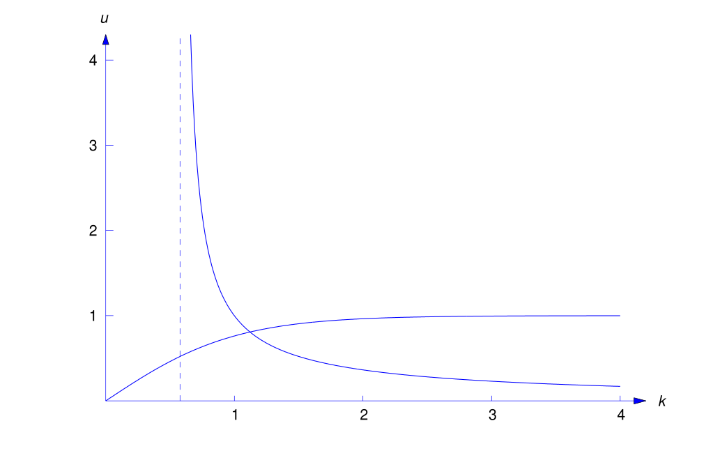
\begin{equation} \tanh k=-\frac{2k}{1-3k^{2}}. \tag{13.2.18}\end{equation}

The graph of the right side (Figure 13.2.1) has a vertical asymptote at \(k=1/\sqrt{3}\). Since the two sides have different signs if \(k<1/\sqrt{3}\), this equation has no solution in \((0,1/\sqrt{3})\). Figure 13.2.1 shows the graphs of the two sides of (13.2.18) on an interval to the right of the vertical asymptote, which is indicated by the dashed line. You can see that the two curves intersect near \(k_{0}=1.2\), Given this estmate, you can use Newton’s to compute \(k_{0}\) more accurately. We computed \(k_{0}\approx 1.1219395\). Therefore \(-k_{0}^{2}\approx -1.2587483\) is an eigenvalue of (13.2.15). From (13.2.16) and the first equation in (13.2.17),

\[ y_{0}=k_{0}\cosh k_{0}x-\sinh k_{0}x. \]

u=k and u=-2k/(1-3k^2) — Figure 13.2.1. \(u=\tanh k\) and \(u=-2k/(1-3k^2)\)

If \(\lambda>0\) we write \(\lambda=k^{2}\) where \(k>0\), and differential equation in (13.2.15) becomes \(y''+k^{2}y=0\), with general solution

\begin{equation} y= \cos kx + c_{2}\sin kx, \tag{13.2.19}\end{equation}

\[ y'=k(-c_{1}\sin kx+c_{2}\cos kx). \]

The boundary conditions require that

\begin{equation} \begin{gathered} c_{1}+kc_{2}=0\\ (\cos k-3k\sin k)c_{1}+(\sin k+3k\cos k)c_{2}=0. \end{gathered} \tag{13.2.20}\end{equation}

The determinant of this system is

\begin{eqnarray*} D_{P}(k)&=& \left|\begin{array}{cccccc} 1&k\\ \cos k-3k\sin k&\sin k+3k \cos k \end{array}\right| \\ &=& (1+3k^{2})\sin k+2k \cos k. \end{eqnarray*}

The system (13.2.20) has a nontrivial solution if and only if \(D_{P}(k)=0\) or, equivalently,

\[ \tan k=-\frac{2k}{1+3k^{2}}. \]

Figure 13.2.2 shows the graphs of the two sides of this equation. You can see from the figure that the graphs intersect at infinitely many points \(k_{n}\approx n\pi\) (\(n=1\), \(2\), \(3\),…), where the error in this approximation approaches zero as \(n\to\infty\). Given this estimate, you can use Newton’s method to compute \(k_{n}\) more accurately. We computed

\begin{eqnarray*} k_{1}&\approx&\phantom{1}2.9256856, \\ k_{2}&\approx&\phantom{1} 6.1765914, \\ k_{3}&\approx&\phantom{1} 9.3538959, \\ k_{4}&\approx& 12.5132570. \end{eqnarray*}

The estimates of the corresponding eigenvalues \(\lambda_{n}=k_{n}^{2}\) are

\begin{eqnarray*} \lambda_{1}&\approx&\phantom{15} 8.5596361, \\ \lambda_{2}&\approx&\phantom{5} 38.1502809, \\ \lambda_{3}&\approx&\phantom{5} 87.4953676, \\ \lambda_{4}&\approx& 156.5815998. \end{eqnarray*}

From (13.2.19) and the first equation in (13.2.20),

\[ y_{n}=k_{n}\cos k_{n}x-\sin k_{n}x \]

is an eigenfunction associated with \(\lambda_{n}\) ∎

u=k and u=-2k/(1+k) — Figure 13.2.2. \(u=\tan k\) and \(u=-2k/(1+k)\)

Since the differential equations in (13.2.12) and (13.2.14) are more complicated than those in (13.2.11) and (13.2.13) respectively, what is the point of Theorem 13.2.1? The point is this: to solve a specific problem, it may be better to deal with it directly, as we did in Examples 13.2.1 and 13.2.2; however, we’ll see that transforming the general eigenvalue problem (13.2.1) to the Sturm–Liouville problem (13.2.10) leads to results applicable to all eigenvalue problems of the form (13.2.1).

Theorem 13.2.2

\[ Ly=(p(x)y')'+q(x)y \]

and \(u\) and \(v\) are twice continuously functions on \([a,b]\) that satisfy the boundary conditions \(B_{1}(y)=0\) and \(B_{2}(y)=0,\) then

\begin{equation} \int_{a}^{b}[u(x)Lv(x)-v(x)Lu(x)]\,dx=0. \tag{13.2.21}\end{equation}

Proof Integration by parts yields

\begin{eqnarray*} \int_{a}^{b}[u(x)Lv(x)-v(x)Lu(x)]\,dx&=& \int_{a}^{b}[u(x)(p(x)v'(x))'-v(x)(p(x)u'(x))']\,dx \\ &=& p(x)[u(x)v'(x)-u'(x)v(x)]\bigg|_{a}^{b} \\ &&-\int_{a}^{b}p(x)[u'(x)v'(x)-u'(x)v'(x)]\,dx. \end{eqnarray*}

Since the last integral equals zero,

\begin{equation} \int_{a}^{b}[u(x)Lv(x)-v(x)Lu(x)]\,dx = p(x)[u(x)v'(x)-u'(x)v'(x)]\bigg|_{a}^{b}. \tag{13.2.22}\end{equation}

By assumption, \(B_{1}(u)=B_{1}(v)=0\) and \(B_{2}(u)=B_{2}(v)=0\). Therefore

\[ \begin{aligned} \alpha u(a)+\beta u'(a)&=0\\ \alpha v(a)+\beta v'(a)&=0\\ \end{aligned} \quad \text{\quad and\quad}\quad \begin{gathered} \rho u(b)+\delta u'(b)=0\phantom{.}\\ \rho v(b)+\delta v'(b)=0. \end{gathered} \]

Since \(\alpha^{2}+\beta^{2}>0\) and \(\rho^{2}+\delta^{2}>0\), the determinants of these two systems must both be zero; that is,

\[ u(a)v'(a)-u'(a)v(a)=u(b)v'(b)-u'(b)v(b)=0. \]

This and (13.2.22) imply (13.2.21), which completes the proof.

The next theorem shows that a Sturm–Liouville problem has no complex eigenvalues.

Theorem 13.2.3

If \(\lambda=p+qi\) with \(q\ne0\) then the boundary value problem

\[ Ly+\lambda r(x)y=0,\quad B_{1}(y)=0,\quad B_{2}(y)=0 \]

has only the trivial solution.

Proof For this theorem to make sense, we must consider complex-valued solutions of

\begin{equation} Ly+(p+iq)r(x,y)y=0. \tag{13.2.23}\end{equation}

If \(y=u+iv\) where \(u\) and \(v\) are real-valued and twice differentiable, we define \(y'=u'+iv'\) and \(y''=u''+iv''\). We say that \(y\) is a solution of (13.2.23) if the real and imaginary parts of the left side of (13.2.23) are both zero. Since \(Ly=(p(x)'y)'+q(x)y\) and \(p\), \(q\), and \(r\) are real-valued,

\begin{eqnarray*} Ly+\lambda r(x)y&=&L(u+iv)+(p+iq)r(x)(u+iv) \\ &=&Lu+r(x)(pu-qv)+i[Lv+r(x)(pu+qv)], \end{eqnarray*}

so \(Ly+\lambda r(x)y=0\) if and only if

\begin{eqnarray*} Lu+r(x)(pu-qv)&=&0 \\ Lv+r(x)(qu+pv)&=&0. \end{eqnarray*}

Multiplying the first equation by \(v\) and the second by \(u\) yields

\begin{eqnarray*} vLu+r(x)(puv-qv^{2})&=&0 \\ uLv+r(x)(qu^{2}+puv)&=&0. \end{eqnarray*}

Subtracting the first equation from the second yields

\[ uLv-vLu+qr(x)(u^{2}+v^{2})=0, \]

\begin{equation} \int_{a}^{b}[u(x)Lv(x)-v(x)Lu(x)]\,dx+ \int_{a}^{b}r(x)[u^{2}(x)+v^{2}(x)]\,dx=0. \tag{13.2.24}\end{equation}

Since

\[ B_{1}(y)=B_{1}(u+iv)=B_{1}(u)+iB_{1}(v) \]

and

\[ B_{2}(y)=B_{2}(u+iv)=B_{2}(u)+iB_{2}(v), \]

\(B_{1}(y)=0\) and \(B_{2}(y)=0\) implies that

\[ B_{1}(u)=B_{2}(u)=B_{1}(v)=B_{2}(v)=0. \]

Therefore Theorem 13.2.2 implies that first integral in (13.2.24) equals zero, so (13.2.24) reduces to

\[ q\int_{a}^{b}r(x)[u^{2}(x)+v^{2}(x)]\,dx =0. \]

Since \(r\) is positive on \([a,b]\) and \(q\ne0\) by assumption, this implies that \(u\equiv0\) and \(v\equiv0\) on \([a,b]\). Therefore \(y\equiv0\) on \([a,b]\), which completes the proof.

Theorem 13.2.4

If \(\lambda_{1}\) and \(\lambda_{2}\) are distinct eigenvalues of the Sturm–Liouville problem

\begin{equation} Ly+\lambda r(x)y=0,\quad B_{1}(y)=0,\quad B_{2}(y)=0 \tag{13.2.25}\end{equation}

with associated eigenfunctions \(u\) and \(v\) respectively\(,\) then

\begin{equation} \int_{a}^{b}r(x)u(x)v(x)\,dx=0. \tag{13.2.26}\end{equation}

Proof Since \(u\) and \(v\) satisfy the boundary conditions in (13.2.25), Theorem 13.2.2 implies that

\[ \int_{a}^{b}[u(x)Lv(x)-v(x)Lu(x)]\,dx=0. \]

Since \(Lu=-\lambda_{1}ru\) and \(Lv=-\lambda_{2}rv\), this implies that

\[ (\lambda_{1}-\lambda_{2})\int_{a}^{b}r(x)u(x)v(x)\,dx=0. \]

Since \(\lambda_{1}\ne\lambda_{2}\), this implies (13.2.26), which completes the proof.

If \(u\) and \(v\) are any integrable functions on \([a,b]\) and

\[ \int_{a}^{b} r(x)u(x)v(x)\,dx=0, \]

we say that \(u\) and \(v\) orthogonal on \([a,b]\) with respect to \(r=r(x)\).

Theorem 13.1.1 implies the next theorem.

Theorem 13.2.5

If \(u\not\equiv0\) and \(v\) both satisfy

\[ Ly+\lambda r(x)y=0,\quad B_{1}(y)=0,\quad B_{2}(y)=0, \]

then \(v=cu\) for some constant \(c.\)

We’ve now proved parts of the next theorem. A complete proof is beyond the scope of this book.

Theorem 13.2.6

The set of all eigenvalues of the Sturm–Liouville problem

\[ Ly+\lambda r(x)y=0,\quad B_{1}(y)=0,\quad B_{2}(y)=0 \]

can be ordered as

\[ \lambda_{1}<\lambda_{2}<\cdots<\lambda_{n}<\cdots, \]

and

\[ \lim_{n\to\infty} \lambda_{n}=\infty. \]

For each \(n,\) if \(y_{n}\) is an arbitrary \(\lambda_{n}\)-eigenfunction\(,\) then every \(\lambda_{n}\)-eigenfunction is a constant multiple of \(y_{n}.\) If \(m\ne n,\) \(y_{m}\) and \(y_{n}\) are orthogonal \([a,b]\) with respect to \(r=r(x);\) that is\(,\)

\begin{equation} \int_{a}^{b} r(x)y_{m}(x)y_{n}(x)\,dx=0. \tag{13.2.27}\end{equation}

You may want to verify (13.2.27) for the eigenfunctions obtained in Examples 13.2.1 and 13.2.2.

In conclusion, we mention the next theorem. The proof is beyond the scope of this book.

Theorem 13.2.7

Let \(\lambda_{1}<\lambda_{2}<\cdots<\lambda_{n}<\cdots\) be the eigenvalues of the Sturm–Liouville problem

\[ Ly+\lambda r(x)y=0,\quad B_{1}(y)=0,\quad B_{2}(y)=0, \]

with associated eigenvectors \(y_{1},\) \(y_{2},\) …, \(y_{n},\) …\(.\) Suppose \(f\) is piecewise smooth \((\)Definition \(\ref{thmtype:11.2.3})\) on \([a,b].\) For each \(n,\) let

\[ c_{n}=\frac{\dst{\int_{a}^{b}}r(x)f(x)y_{n}(x)\,dx} {\dst{\int_{a}^{b}}r(x)y_{n}^{2}(x)\,dx}. \]

Then

\[ \frac{f(x-)+f(x+)}{2}=\sum_{n=1}^{\infty}c_{n}y_{n}(x) \]

for all \(x\) in the open interval \((a,b).\)

13.2 Exercises

In Exercises \(\ref{exer:13.2.1}\)–\(\ref{exer:13.2.7}\) rewrite the equation in Sturm–Liouville form \((\)with \(\lambda=0)\). Assume that \(b,\) \(c,\) \(\alpha,\) and \(\nu\) are contants\(.\)

\(y''+by'+cy=0\)

Show answer

\((e^{bx}y')'+ce^{bx}y=0\)
\(x^{2}y''+xy'+(x^{2}-\nu^{2})y=0\) (Bessel’s equation)

Show answer

\(\dst{(xy')'+\left(x-\frac{\nu^{2}}{x}\right)y=0}\)
\((1-x^{2})y''-xy'+\alpha^{2}y=0\) (Chebyshev’s equation)

Show answer

\(\dst{(\sqrt{1-x^{2}}y')'+\frac{\alpha^{2}}{\sqrt{1-x^{2}}}y=0}\)
\(x^{2}y''+bxy'+cy=0\) (Euler’s equation)

Show answer

\((x^{b}y')'+cx^{b-2}y=0\)
\(y''-2xy'+2\alpha y=0\) (Hermite’s equation)

Show answer

\((e^{-x^{2}}y')'+2\alpha e^{-x^{2}}y =0\)
\(xy''+(1-x)y'+\alpha y=0\) (Laguerre’s equation)

Show answer

\((xe^{-x}y')'+\alpha e^{-x}y=0\)
\((1-x^{2})y''-2xy'+\alpha(\alpha+1)y=0\) (Legendre’s equation)

Show answer

\(((1-x^{2})y')'+\alpha(\alpha+1)y=0\)
In Example 13.2.4 we found that the eigenvalue problem

\begin{equation} x^{2}y''+xy'+\lambda y=0,\quad y(1)=0,\quad y(2)=0 \tag{A} \end{equation}

is equivalent to the Sturm-Liouville problem

\begin{equation} \tag{B} (xy')'+\frac{\lambda}{x}y=0,\quad y(1)=0,\quad y(2)=0. \end{equation}

Multiply the differential equation in (B) by \(y\) and integrate to show that

\[ \lambda\int_{1}^{2}\frac{y^{2}(x)}{x}\,dx=\int_{1}^{2}x(y'(x))^{2}\,dx. \]

Conclude from this that the eigenvalues of (A) are all positive.
Solve the eigenvalue problem

\[ y''+2y'+y+\lambda y=0,\quad y(0)=0, \quad y(1)=0. \]

Show answer

\(\lambda_{n}=n^{2}\pi^{2}\), \(y_{n}=e^{-x}\sin n\pi x\) (\(n=\) positive integer)
Solve the eigenvalue problem

\[ y''+2y'+y+\lambda y=0,\quad y'(0)=0, \quad y'(1)=0. \]

Show answer

\(\lambda_{0}=-1\), \(y_{0}=1\) \(\lambda_{n}=n^{2}\pi^{2}\), \(y_{n}=e^{-x}(n\pi\cos n\pi x+\sin n\pi x)\) (\(n=\) positive

integer)

In Exercises \(\ref{exer:13.2.11}\)–\(\ref{exer:13.2.20}:\) (a) Determine whether \(\lambda=0\) is an eigenvalue. If it is, find an associated eigenfunction.

(b) Compute the negative eigenvalues with errors not greater than \(5\times 10^{-8}\). State the form of the associated eigenfunctions.

(c) Compute the first four positive eigenvalues with errors not greater than \(5\times 10^{-8.}\) State the form of the associated eigenfunctions.

C \(y''+\lambda y=0\), \(y(0)+2y'(0)=0\), \(y(2)=0\)

Show answer

(a) \(\lambda=0\) is an eigenvalue \(y_{0}=2-x\) (b) none (c) \(5.0476821\), \(14.9198790\),

\(29.7249673\), \(49.4644528\) \(y=2\sqrt{\lambda}\cos\sqrt{\lambda}\,x-\sin\sqrt{\lambda} x\)
C \(y''+\lambda y=0\), \(y'(0)=0\), \(y(1)-2y'(1)=0\)

Show answer

(a) \(\lambda=0\) isn’t an eigenvalue (b) \(-0.5955245\) \(y=\cosh \sqrt{-\lambda}\,x\) (c) \(8.8511386\),

\(38.4741053\), \(87.8245457\), \(156.9126094\) \(y=\cos\sqrt\lambda x\)
C \(y''+\lambda y=0\), \(y(0)-y'(0)=0\), \(y'(\pi)=0\)

Show answer

(a) \(\lambda=0\) isn’t an eigenvalue (b) none (c) \(0. 1470328\), \(1.4852833\), \(4.5761411\),

\(9.6059439 \) \(y=\sqrt\lambda\cos\sqrt\lambda x+\sin\sqrt\lambda x\)
C \(y''+\lambda y=0\), \(y(0)+2y'(0)=0\), \(y(\pi)=0\)

Show answer

(a) \(\lambda=0\) isn’t an eigenvalue (b) \(-0.1945921\)

\(y=2\sqrt{-\lambda}\,\cosh \sqrt{-\lambda}\,x\; -\sinh\sqrt{-\lambda}\,x\) (c) \(1.9323619\), \(5.9318981\), \(11.9317920\),

\(19.9317507\) \(y=2\sqrt{\lambda}\,\cos \sqrt{\lambda}\,x-\sin\sqrt{\lambda}\,x\)
C \(y''+\lambda y=0\), \(y'(0)=0\), \(y(2)-y'(2)=0\)

Show answer

(a) \(\lambda=0\) isn’t an eigenvalue (b) \(-1.0664054\) \(y=\cosh\sqrt{-\lambda}\,x\) (c) \(1.5113188\),

\(8.8785880\), \(21.2104662\), \(38.4805610\) \(y=\cos\sqrt{\lambda}\,x\)
C \(y''+\lambda y=0\), \(y(0)+y'(0)=0\), \(y(2)+2y'(2)=0\)

Show answer

(a) \(\lambda=0\) isn’t an eigenvalue (b) \(-1.0239346\)

\(y=\sqrt{-\lambda}\,\cosh \sqrt{-\lambda}\,x\; -\sinh\sqrt{-\lambda}\,x\) (c) \(2.0565705\), \(9.3927144\), \(21.7169130\),

\(38.9842177\) \(y=\sqrt{\lambda}\,\cos \sqrt{\lambda}\,x-\sin\sqrt{\lambda}\,x\)
C \(y''+\lambda y=0\), \(y(0)+2y'(0)=0\), \(y(3)-2y'(3)=0\)

Show answer

(a) \(\lambda=0\) isn’t an eigenvalue (b) \(-0.4357577\),

\(y=2\sqrt{-\lambda}\,\cosh \sqrt{-\lambda}\,x\; -\sinh\sqrt{-\lambda}\,x\) (c) \(0.3171423\), \(3.7055350\), \(9.1970150\),

\(16.8760401\) \(y=2\sqrt{\lambda}\,\cos \sqrt{\lambda}\,x-\sin\sqrt{\lambda}\,x\)
C \(y''+\lambda y=0\), \(3y(0)+y'(0)=0\), \(3y(2)-2y'(2)=0\)

Show answer

(a) \(\lambda=0\) isn’t an eigenvalue (b) \(-2.1790546\), \(-9.0006633\)

\(y=\sqrt{-\lambda}\,\cosh\sqrt{-\lambda}\,x-3\sinh\sqrt{-\lambda}\,x\)

(c) \(5.8453181\), \(17.9260967\), \(35.1038567\), \(57.2659330\) \(y=\sqrt{\lambda}\,\cos\sqrt{\lambda}\,x-3\sin\sqrt{\lambda}\,x\)
C \(y''+\lambda y=0\), \(y(0)+2y'(0)=0\), \(y(3)-y'(3)=0\)

Show answer

(a) \(\lambda=0\) is an eigenvalue \(y_{0}=2-x\) (b) \(-1.0273046 \)

\(y=2\sqrt{-\lambda}\,\cosh\sqrt{-\lambda}\,x-\sinh\sqrt{-\lambda}\,x\) (c) \(8.8694608\), \(16.5459202\), \(26.4155505\),

\(38.4784094\) \(y=2\sqrt{\lambda}\,\cos\sqrt{\lambda}\,x-\sin\sqrt{\lambda}\,x\)
C \(y''+\lambda y=0\), \(5y(0)+2y'(0)=0\), \(5y(1)-2y'(1)=0\)

Show answer

(a) \(\lambda=0\) isn’t an eigenvalue (b) \(-7.9394171\), \(-3.1542806\)

\(y=2\sqrt{-\lambda}\,\cosh\sqrt{-\lambda}\,x-5\sinh\sqrt{-\lambda}\,x\) (c) \(29.3617465\), \(78.777456\), \(147.8866417\),

\(236.7229622\) \(y=2\sqrt{\lambda}\,\cos\sqrt{\lambda}\,x-5\sin\sqrt{\lambda}\,x\)
Find the first five eigenvalues of the boundary value problem

\[ y''+2y'+y+\lambda y=0,\quad y(0)=0,\quad y'(1)=0 \]

with errors not greater than \(5\times 10^{-8}\). State the form of the associated eigenfunctions.

Show answer

\(\lambda=0\), \(y=xe^{-x}\) \(20.1907286\), \(118.8998692\), \(296.5544121\), \(553.1646458\)

\(y=e^{-x}\sin\sqrt{\lambda}\,x\)

In Exercises 22–24 take it as given that \(\{xe^{kx},xe^{-kx}\}\) and \(\{x\cos kx, x\sin kx\}\) are fundamental sets of solutions of

\[ x^{2}y''-2xy'+2y-k^{2}x^{2}y=0 \]

and

\[ x^{2}y''-2xy'+2y+k^{2}x^{2}y=0, \]

respectively.

Solve the eigenvalue problem for

\[ x^{2}y''-2xy'+2y+\lambda x^{2}y=0, \quad y(1)=0,\quad y(2)=0. \]

Show answer

\(\lambda_{n}=n^{2}\pi^{2}\), \(y_{n}=x\sin n\pi(x-2)\) (\(n=\) positive integer)
C Find the first five eigenvalues of

\[ x^{2}y''-2xy'+2y+\lambda x^{2}y=0, \quad y'(1)=0,\quad y(2)=0 \]

with errors no greater than \(5\times 10^{-8}\). State the form of the associated eienfunctions.

Show answer

\(\lambda=0\), \(y=x(2-x)\) \(20.1907286\), \(118.8998692\), \(296.5544121\)

\(553.1646458\), \(y=x\sin\sqrt{\lambda}\,(x-2)\)
C Find the first five eigenvalues of

\[ x^{2}y''-2xy'+2y+\lambda x^{2}y=0, \quad y(1)=0,\quad y'(2)=0 \]

with errors no greater than \(5\times 10^{-8}\). State the form of the associated eienfunctions.

Show answer

\(3.3730893\), \(23.1923372\), \(62.6797232\), \(121.8999231\), \(200.8578309\)

\(y=x\sin\sqrt{\lambda}\,(x-1)\)
Consider the Sturm-Liouville problem

\begin{equation} \tag{A} y''+\lambda y=0,\quad y(0)=0,\quad y(L)+\delta y'(L)=0. \end{equation}

(a) Show that (A) can’t have more than one negative eigenvalue, and find the values of \(\delta\) for which it has one.

(b) Find all values of \(\delta\) such that \(\lambda=0\) is an eigenvalue of (A).

(c) Show that \(\lambda=k^{2}\) with \(k>0\) is an eigenvalue of (A) if and only if

\begin{equation} \tag{B} \tan kL=-\delta k. \end{equation}

(d) For \(n=1\), \(2\), …, let \(y_{n}\) be an eigenfunction associated with \(\lambda_{n}=k_{n}^{2}\). From Theorem 13.2.4, \(y_{m}\) and \(y_{n}\) are orthogonal over \([0,L]\) if \(m\ne n\). Verify this directly. Hint: Integrate by parts twice and use (B).

Show answer

(a) \(-L<\delta<0\) (b) \(\delta=-L\)
Solve the Sturm-Liouville problem

\[ y''+\lambda y=0,\quad y(0)+\alpha y'(0)=0,\quad y(\pi)+\alpha y'(\pi)=0, \]

where \(\alpha\ne0\).

Show answer

\(\lambda_{0}=-1/\alpha^{2}\) \(y_{0}=e^{-x/\alpha}\) \(\lambda_{n}=n^{2}\), \(y_{n}=n\alpha \cos nx-\sin nx\), \(n=1\), \(2\), …
L Consider the Sturm-Liouville problem

\begin{equation} \tag{A} y''+\lambda y=0,\quad y(0)+\alpha y'(0)=0,\quad y(1)+(\alpha-1) y'(1)=0, \end{equation}

where \(0<\alpha<1\).

(a) Show that \(\lambda=0\) is an eigenvalue of (A), and find an associated eigenfunction.

(b) Show that (A) has a negative eigenvalue, and find the form of an associated eigenfunction.

(c) Give a graphical argument to show that (A) has infinitely many positive eigenvalues \(\lambda_{1} < \lambda_{2}<\cdots <\lambda_{n}<\cdots\), and state the form of the associated eigenfunctions.

Show answer

(a) \(y=x-\alpha\) (b) \(y=\alpha k\cosh kx-\sin kx\) (c) \(y=\alpha k\cos kx-\sin kx\)

Exercises 28–30 deal with the Sturm–Liouville problem

\begin{equation} \tag{SL} y''+\lambda y=0,\quad \alpha y(0)+\beta y'(0),\quad \rho y(L)+\delta y'(L)=0, \end{equation}

where \(\alpha^{2}+\beta^{2}>0\) and \(\rho^{2}+\delta^{2}>0\).

Show that \(\lambda=0\) is an eigenvalue of (SL) if and only if

\[ \alpha(\rho L+\delta)-\beta\rho =0. \]
L The point of this exercise is that (SL) can’t have more than two negative eigenvalues.

(a) Show that \(\lambda\) is a negative eigenvalue of (SL) if and only if \(\lambda=-k^{2}\), where \(k\) is a positive solution of

\[ (\alpha\rho-\beta\delta k^{2})\sinh kL+k(\alpha\delta-\beta\rho)\cosh kL. \]

(b) Suppose \(\alpha\delta-\beta\rho=0\). Show that (SL) has a negative eigenvalue if and only if \(\alpha\rho\) and \(\beta\delta\) are both nonzero. Find the negative eigenvalue and an associated eigenfunction. Hint: Show that in this case \(\rho=p\alpha\) and \(s=q\beta\), where \(q\ne0\).

(c) Suppose \(\beta\rho-\alpha\delta\ne0\). We know from Section 11.1 that (SL) has no negative eigenvalues if \(\alpha\rho=0\) and \(\beta\delta=0\). Assume that either \(\alpha\rho\ne0\) or \(\beta\delta\ne0\). Then we can rewrite (A) as

\[ \tanh kL= \frac{k(\beta\rho-\alpha\delta)}{\alpha\rho-\beta\delta k^{2}}. \]

By graphing both sides of this equation on the same axes (there are several possibilities for the right side), show that it has at most two positive solutions, so (SL) has at most two negative eigenvalues.

Show answer

(b) \(\lambda=-\alpha^{2}/\beta^{2}\) \(y=e^{-\alpha x/\beta}\)
L The point of this exercise is that (SL) has infinitely many positive eigenvalues \(\lambda_{1}<\lambda_{2}<\cdots<\lambda_{n}<\cdots\), and that \(\lim_{n\to\infty}\lambda_{n}=\infty\).

(a) Show that \(\lambda\) is a positive eigenvalue of (SL) if and only if \(\lambda=k^{2}\), where \(k\) is a positive solution of

\begin{equation} \tag{A} (\alpha\rho+\beta\delta k^{2})\sin kL+k(\alpha\delta-\beta\rho)\cos kL=0. \end{equation}

(b) Suppose \(\alpha\delta-\beta\rho=0\). Show that the positive eigenvalues of (SL) are \(\lambda_{n}=(n\pi/L)^{2}\), \(n=1\), \(2\), \(3\), …. Hint: Recall the hint in Exercise 29(b).

Now suppose \(\alpha\delta-\beta\rho\ne0\). From Section 11.1, if \(\alpha\rho=0\) and \(\beta\delta=0\), then (SL) has the eigenvalues

\[ \lambda_{n}=[(2n-1)\pi/2L]^{2},\quad n=1,2,3, \dots \]

(why?), so let’s suppose in addition that at least one of the products \(\alpha\rho\) and \(\beta\delta\) is nonzero. Then we can rewrite (A) as

\begin{equation} \tag{B} \tan kL= \frac{k(\beta\rho-\alpha\delta)} {\alpha\rho-\beta\delta k^{2}}. \end{equation}

By graphing both sides of this equation on the same axes (there are several possibilities for the right side), convince yourself of the following:

(c) If \(\beta\delta=0\), there’s a positive integer \(N\) such that (B) has one solution \(k_{n}\) in each of the intervals

\begin{equation} \tag{C} \left((2n-1)\pi/L, (2n+1)\pi/L)\right),\quad n=N,N+1,N+2,\dots, \end{equation}

and either

\[ \lim_{n\to\infty}\left(k_{n}-\frac{(2n-1)\pi}{2L}\right) =0 \text{\quad or\quad} \lim_{n\to\infty}\left(k_{n}-\frac{(2n+1)\pi}{2L}\right)=0. \]

(d) If \(\beta\delta\ne0\), there’s a positive integer \(N\) such that (B) has one solution \(k_{n}\) in each of the intervals (C) and

\[ \lim_{n\to\infty}\left(k_{n}-\frac{n\pi}{N}\right)=0. \]
The following Sturm–Liouville problems are genera1izations of Problems 1–4 of Section 11.1.

Problem 1: \((p(x)y')'+\lambda r(x)y=0\), \(y(a)=0\), \(y(b)=0\)

Problem 2: \((p(x)y')'+\lambda r(x)y=0\), \(y'(a)=0\), \(y'(b)=0\)

Problem 3: \((p(x)y')'+\lambda r(x)y=0\), \(y(a)=0\), \(y'(b)=0\)

Problem 4: \((p(x)y')'+\lambda r(x)y=0\), \(y'(a)=0\), \(y(b)=0\)

Prove: Problems 1–4 have no negative eigenvalues. Moreover, \(\lambda=0\) is an eigenvalue of Problem 2 with associated eigenfunction \(y_{0}=1\), but \(\lambda=0\) isn’t an eigenvalue of Problems 1, 3, and 4. Hint: See the proof of Theorem 11.1.1.
Show that the eigenvalues of the Sturm–Liouville problem

\[ (p(x)y')'+\lambda r(x)y=0,\quad \alpha y(a)+ \beta y'(a)=0,\quad \rho y(b)+\delta y'(b) \]

are all positive if \(\alpha\beta\le 0\), \(\rho\delta\ge 0\), and \((\alpha\beta)^{2}+(\rho\delta)^{2}>0\).