4.8 Lagrange Multipliers

Use the method of Lagrange multipliers to solve optimization problems with one constraint.
Use the method of Lagrange multipliers to solve optimization problems with two constraints.

Solving optimization problems for functions of two or more variables can be similar to solving such problems in single-variable calculus. However, techniques for dealing with multiple variables allow us to solve more varied optimization problems for which we need to deal with additional conditions or constraints. In this section, we examine one of the more common and useful methods for solving optimization problems with constraints.

Lagrange Multipliers

Example 4.41 was an applied situation involving maximizing a profit function, subject to certain constraints. In that example, the constraints involved a maximum number of golf balls that could be produced and sold in $1$ month $(x),$ and a maximum number of advertising hours that could be purchased per month $(y) .$ Suppose these were combined into a budgetary constraint, such as $20 x + 4 y \leq 216,$ that took into account the cost of producing the golf balls and the number of advertising hours purchased per month. The goal is, still, to maximize profit, but now there is a different type of constraint on the values of $x$ and $y .$ This constraint, when combined with the profit function $f (x, y) = 48 x + 96 y - x^{2} - 2 x y - 9 y^{2},$ is an example of an optimization problem, and the function $f (x, y)$ is called the objective function. A graph of various level curves of the function $f (x, y)$ follows.

A series of rotated ellipses that become increasingly large. The smallest one is marked f(x, y) = 400, and the biggest one is marked f(x, y) = 150. — Figure 4.59 Graph of level curves of the function $f (x, y) = 48 x + 96 y - x^{2} - 2 x y - 9 y^{2}$ corresponding to $c = 150, 250, 350, and 400 .$

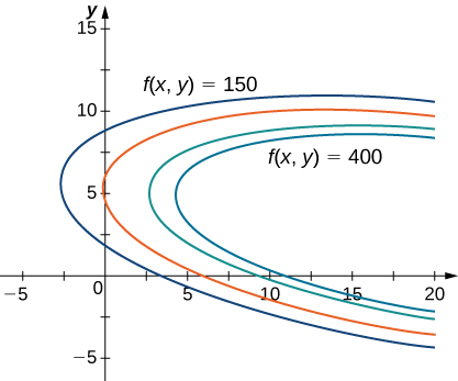
In Figure 4.59, the value $c$ represents different profit levels (i.e., values of the function $f) .$ As the value of $c$ increases, the curve shifts to the right. Since our goal is to maximize profit, we want to choose a curve as far to the right as possible. If there was no restriction on the number of golf balls the company could produce, or the number of units of advertising available, then we could produce as many golf balls as we want, and advertise as much as we want, and there would not be a maximum profit for the company. Unfortunately, we have a budgetary constraint that is modeled by the inequality $20 x + 4 y \leq 216 .$ To see how this constraint interacts with the profit function, Figure 4.60 shows the graph of the line $20 x + 4 y = 216$ superimposed on the previous graph.

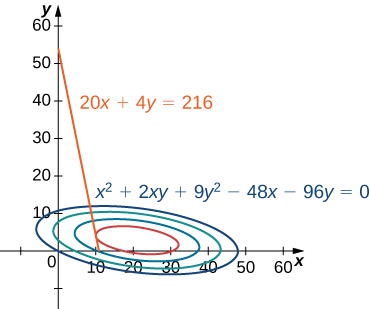
A series of rotated ellipses that become increasingly large. On the smallest ellipse, which is red, there is a tangent line marked with equation 20x + 4y = 216 that appears to touch the ellipse near (10, 4). — Figure 4.60 Graph of level curves of the function $f (x, y) = 48 x + 96 y - x^{2} - 2 x y - 9 y^{2}$ corresponding to $c = 150, 250, 350, and 395 .$ The red graph is the constraint function.

As mentioned previously, the maximum profit occurs when the level curve is as far to the right as possible. However, the level of production corresponding to this maximum profit must also satisfy the budgetary constraint, so the point at which this profit occurs must also lie on (or to the left of) the red line in Figure 4.60. Inspection of this graph reveals that this point exists where the line is tangent to the level curve of $f .$ Trial and error reveals that this profit level seems to be around $395,$ when $x$ and $y$ are both just less than $5 .$ We return to the solution of this problem later in this section. From a theoretical standpoint, at the point where the profit curve is tangent to the constraint line, the gradient of both of the functions evaluated at that point must point in the same (or opposite) direction. Recall that the gradient of a function of more than one variable is a vector. If two vectors point in the same (or opposite) directions, then one must be a constant multiple of the other. This idea is the basis of the method of Lagrange multipliers.

Method of Lagrange Multipliers: One Constraint

Let $f$ and $g$ be functions of two variables with continuous partial derivatives at every point of some open set containing the smooth curve $g (x, y) = 0 .$ Suppose that $f,$ when restricted to points on the curve $g (x, y) = 0,$ has a local extremum at the point $(x_{0}, y_{0})$ and that $\nabla g (x_{0}, y_{0}) \neq 0 .$ Then there is a number $λ$ called a Lagrange multiplier, for which

\nabla f (x_{0}, y_{0}) = λ \nabla g (x_{0}, y_{0}) .

Proof

Assume that a constrained extremum occurs at the point $(x_{0}, y_{0}) .$ Furthermore, we assume that the equation $g (x, y) = 0$ can be smoothly parameterized as

x = x (s) and y = y (s)

where s is an arc length parameter with reference point $(x_{0}, y_{0})$ at $s = 0 .$ Therefore, the quantity $z = f (x (s), y (s))$ has a relative maximum or relative minimum at $s = 0,$ and this implies that $\frac{d z}{d s} = 0$ at that point. From the chain rule,

\frac{d z}{d s} = \frac{\partial f}{\partial x} \cdot \frac{d x}{d s} + \frac{\partial f}{\partial y} \cdot \frac{d y}{d s} = (\frac{\partial f}{\partial x} \hat{i} + \frac{\partial f}{\partial y} \hat{j}) \cdot (\frac{d x}{d s} \hat{i} + \frac{d y}{d s} \hat{j}) = 0,

where the derivatives are all evaluated at $s = 0 .$ However, the first factor in the dot product is the gradient of $f,$ and the second factor is the unit tangent vector $T (0)$ to the constraint curve. Since the point $(x_{0}, y_{0})$ corresponds to $s = 0,$ it follows from this equation that

\nabla f (x_{0}, y_{0}) \cdot T (0) = 0,

which implies that the gradient is either $0$ or is normal to the constraint curve at a constrained relative extremum. However, the constraint curve $g (x, y) = 0$ is a level curve for the function $g (x, y)$ so that if $\nabla g (x_{0}, y_{0}) \neq 0$ then $\nabla g (x_{0}, y_{0})$ is normal to this curve at $(x_{0}, y_{0})$ It follows, then, that there is some scalar $λ$ such that

\nabla f (x_{0}, y_{0}) = λ \nabla g (x_{0}, y_{0})

□

To apply Lagrange Multipliers to an optimization problem similar to that for the golf ball manufacturer, we need a problem-solving strategy.

Steps for Using Lagrange Multipliers

Determine the objective function $f (x, y)$ and the constraint function $g (x, y) .$ Does the optimization problem involve maximizing or minimizing the objective function?
Set up a system of equations using the following template:

$\begin{matrix} \nabla f (x_{0}, y_{0}) & = & λ \nabla g (x_{0}, y_{0}) \\ g (x_{0}, y_{0}) & = & 0 . \end{matrix}$
Solve for $x_{0}$ and $y_{0} .$
The largest of the values of $f$ at the solutions found in step $3$ maximizes $f;$ the smallest of those values minimizes $f .$

Using Lagrange Multipliers

Use the method of Lagrange multipliers to find the minimum value of $f (x, y) = x^{2} + 4 y^{2} - 2 x + 8 y$ subject to the constraint $x + 2 y = 7 .$

Let’s follow the problem-solving strategy:

The optimization function is $f (x, y) = x^{2} + 4 y^{2} - 2 x + 8 y .$ To determine the constraint function, we must first subtract $7$ from both sides of the constraint. This gives $x + 2 y - 7 = 0 .$ The constraint function is equal to the left-hand side, so $g (x, y) = x + 2 y - 7 .$ The problem asks us to solve for the minimum value of $f,$ subject to the constraint (see the following graph).

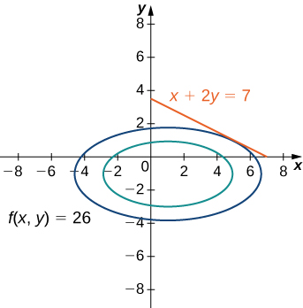
Figure 4.61 Graph of level curves of the function $f (x, y) = x^{2} + 4 y^{2} - 2 x + 8 y$ corresponding to $c = 10$ and $26 .$ The red graph is the constraint function.
We then must calculate the gradients of both f and g:

$\begin{matrix} \nabla f (x, y) = (2 x - 2) i + (8 y + 8) j \\ \nabla g (x, y) = i + 2 j . \end{matrix}$

The equation $\nabla f (x_{0}, y_{0}) = λ \nabla g (x_{0}, y_{0})$ becomes

$(2 x_{0} - 2) i + (8 y_{0} + 8) j = λ (i + 2 j),$

which can be rewritten as

$(2 x_{0} - 2) i + (8 y_{0} + 8) j = λ i + 2λ j .$

Next, we set the coefficients of $i and j$ equal to each other:

$\begin{matrix} 2 x_{0} - 2 = λ \\ 8 y_{0} + 8 = 2 λ . \end{matrix}$

The equation $g (x_{0}, y_{0}) = 0$ becomes $x_{0} + 2 y_{0} - 7 = 0 .$ Therefore, the system of equations that needs to be solved is

$\begin{matrix} 2 x_{0} - 2 & = & λ \\ 8 y_{0} + 8 & = & 2 λ \\ x_{0} + 2 y_{0} - 7 & = & 0. \end{matrix}$
This is a linear system of three equations in three variables. We start by solving the second equation for $λ$ and substituting it into the first equation. This gives $λ = 4 y_{0} + 4,$ so substituting this into the first equation gives

$2 x_{0} - 2 = 4 y_{0} + 4 .$

Solving this equation for $x_{0}$ gives $x_{0} = 2 y_{0} + 3 .$ We then substitute this into the third equation:
$\begin{matrix} (2 y_{0} + 3) + 2 y_{0} - 7 & = & 0 \\ 4 y_{0} - 4 & = & 0 \\ y_{0} & = & 1. \end{matrix}$

Since $x_{0} = 2 y_{0} + 3,$ this gives $x_{0} = 5 .$
Next, we substitute $(5, 1)$ into $f (x, y) = x^{2} + 4 y^{2} - 2 x + 8 y,$ gives $f (5, 1) = 5^{2} + 4 {(1)}^{2} - 2 (5) + 8 (1) = 27 .$ To ensure this corresponds to a minimum value on the constraint function, let’s try some other values, such as the intercepts of $g (x, y) = 0,$ Which are $(7, 0)$ and $(0, 3.5) .$ We get $f (7, 0) = 35$ and $f (0, 3.5) = 77,$ so it appears $f$ has a minimum at $(5, 1) .$

Use the method of Lagrange multipliers to find the maximum value of $f (x, y) = 9 x^{2} + 36 x y - 4 y^{2} - 18 x - 8 y$ subject to the constraint $3 x + 4 y = 32 .$

$f$ has a maximum value of $976$ at the point $(8, 2) .$

Hint

Use the problem-solving strategy for the method of Lagrange multipliers.

Let’s now return to the problem posed at the beginning of the section.

Golf Balls and Lagrange Multipliers

The golf ball manufacturer, Pro-T, has developed a profit model that depends on the number $x$ of golf balls sold per month (measured in thousands), and the number of hours per month of advertising y, according to the function

z = f (x, y) = 48 x + 96 y - x^{2} - 2 x y - 9 y^{2},

where $z$ is measured in thousands of dollars. The budgetary constraint function relating the cost of the production of thousands golf balls and advertising units is given by $20 x + 4 y = 216 .$ Find the values of $x$ and $y$ that maximize profit, and find the maximum profit.

Again, we follow the problem-solving strategy:

The optimization function is $f (x, y) = 48 x + 96 y - x^{2} - 2 x y - 9 y^{2} .$ To determine the constraint function, we first subtract 216 from both sides of the constraint, then divide both sides by $4,$ which gives $5 x + y - 54 = 0 .$ The constraint function is equal to the left-hand side, so $g (x, y) = 5 x + y - 54 .$ The problem asks us to solve for the maximum value of $f,$ subject to this constraint.
So, we calculate the gradients of both $f and$ $g :$

$\begin{matrix} \nabla f (x, y) = (48 - 2 x - 2 y) i + (96 - 2 x - 18 y) j \\ \nabla g (x, y) = 5 i + j . \end{matrix}$

The equation $\nabla f (x_{0}, y_{0}) = λ \nabla g (x_{0}, y_{0})$ becomes

$(48 - 2 x_{0} - 2 y_{0}) i + (96 - 2 x_{0} - 18 y_{0}) j = λ (5 i + j),$

which can be rewritten as

$(48 - 2 x_{0} - 2 y_{0}) i + (96 - 2 x_{0} - 18 y_{0}) j = λ 5 i + λ j .$

We then set the coefficients of $i and j$ equal to each other:

$\begin{matrix} 48 - 2 x_{0} - 2 y_{0} & = & 5 λ \\ 96 - 2 x_{0} - 18 y_{0} & = & λ . \end{matrix}$

The equation $g (x_{0}, y_{0}) = 0$ becomes $5 x_{0} + y_{0} - 54 = 0 .$ Therefore, the system of equations that needs to be solved is

$\begin{matrix} 48 - 2 x_{0} - 2 y_{0} & = & 5 λ \\ 96 - 2 x_{0} - 18 y_{0} & = & λ \\ 5 x_{0} + y_{0} - 54 & = & 0. \end{matrix}$
We use the left-hand side of the second equation to replace $λ$ in the first equation:

$\begin{matrix} 48 - 2 x_{0} - 2 y_{0} & = & 5 (96 - 2 x_{0} - 18 y_{0}) \\ 48 - 2 x_{0} - 2 y_{0} & = & 480 - 10 x_{0} - 90 y_{0} \\ 8 x_{0} & = & 432 - 88 y_{0} \\ x_{0} & = & 54 - 11 y_{0} . \end{matrix}$

Then we substitute this into the third equation:

$\begin{matrix} 5 (54 - 11 y_{0}) + y_{0} - 54 & = & 0 \\ 270 - 55 y_{0} + y_{0} & = & 0 \\ 216 - 54 y_{0} & = & 0 \\ y_{0} & = & 4. \end{matrix}$

Since $x_{0} = 54 - 11 y_{0},$ this gives $x_{0} = 10 .$
We then substitute $(10, 4)$ into $f (x, y) = 48 x + 96 y - x^{2} - 2 x y - 9 y^{2},$ which gives

$\begin{matrix} f (10, 4) & = 48 (10) + 96 (4) - {(10)}^{2} - 2 (10) (4) - 9 {(4)}^{2} \\ = 480 + 384 - 100 - 80 - 144 = 540. \end{matrix}$

Therefore the maximum profit that can be attained, subject to budgetary constraints, is $$ 540,000$ with a production level of $10,000$ golf balls and $4$ hours of advertising bought per month. Let’s check to make sure this truly is a maximum. The endpoints of the line that defines the constraint are $(10.8, 0)$ and $(0, 54)$ Let’s evaluate $f$ at both of these points:

$\begin{matrix} f (10.8, 0) & = & 48 (10.8) + 96 (0) - {10.8}^{2} - 2 (10.8) (0) - 9 (0^{2}) = 401.76 \\ f (0, 54) & = & 48 (0) + 96 (54) - 0^{2} - 2 (0) (54) - 9 (54^{2}) = −21, 060. \end{matrix}$

The second value represents a loss, since no golf balls are produced. Neither of these values exceed $540,$ so it seems that our extremum is a maximum value of $f .$

A company has determined that its production level is given by the Cobb-Douglas function $f (x, y) = 2.5 x^{0.45} y^{0.55}$ where x represents the total number of labor hours in $1$ year and y represents the total capital input for the company. Suppose $1$ unit of labor costs $$ 40$ and $1$ unit of capital costs $$ 50 .$ Use the method of Lagrange multipliers to find the maximum value of $f (x, y) = 2.5 x^{0.45} y^{0.55}$ subject to a budgetary constraint of $$ 500,000$ per year.

A maximum production level of $13890$ occurs with $5625$ labor hours and $$ 5500$ of total capital input.

Hint

Use the problem-solving strategy for the method of Lagrange multipliers.

In the case of an optimization function with three variables and a single constraint function, it is possible to use the method of Lagrange multipliers to solve an optimization problem as well. An example of an optimization function with three variables could be the Cobb-Douglas function in the previous example: $f (x, y, z) = x^{0.2} y^{0.4} z^{0.4},$ where $x$ represents the cost of labor, $y$ represents capital input, and $z$ represents the cost of advertising. The method is the same as for the method with a function of two variables; the equations to be solved are

\begin{matrix} \nabla f (x, y, z) & = & λ \nabla g (x, y, z) \\ g (x, y, z) & = & 0. \end{matrix}

Lagrange Multipliers with a Three-Variable Optimization Function

Find the minimum of the function $f (x, y, z) = x^{2} + y^{2} + z^{2}$ subject to the constraint $x + y + z = 1 .$

The optimization function is $f (x, y, z) = x^{2} + y^{2} + z^{2} .$ To determine the constraint function, we subtract $1$ from each side of the constraint: $x + y + z - 1 = 0$ which gives the constraint function as $g (x, y, z) = x + y + z - 1 .$
Next, we calculate $\nabla f (x, y, z)$ and $\nabla g (x, y, z) :$

$\begin{matrix} \nabla f (x, y, z) = 〈 2 x, 2 y, 2 z 〉 \\ \nabla g (x, y, z) = 〈 1, 1, 1 〉 . \end{matrix}$

This leads to the equations

$\begin{matrix} 〈 2 x_{0}, 2 y_{0}, 2 z_{0} 〉 & = & λ 〈 1, 1, 1 〉 \\ x_{0} + y_{0} + z_{0} - 1 & = & 0 \end{matrix}$

which can be rewritten in the following form:

$\begin{matrix} 2 x_{0} & = & λ \\ 2 y_{0} & = & λ \\ 2 z_{0} & = & λ \\ x_{0} + y_{0} + z_{0} - 1 & = & 0. \end{matrix}$
Since each of the first three equations has $λ$ on the right-hand side, we know that $2 x_{0} = 2 y_{0} = 2 z_{0}$ and all three variables are equal to each other. Substituting $y_{0} = x_{0}$ and $z_{0} = x_{0}$ into the last equation yields $3 x_{0} - 1 = 0,$ so $x_{0} = \frac{1}{3}$ and $y_{0} = \frac{1}{3}$ and $z_{0} = \frac{1}{3}$ which corresponds to a critical point on the constraint curve.
Then, we evaluate f at the point $(\frac{1}{3}, \frac{1}{3}, \frac{1}{3}) :$

$f (\frac{1}{3}, \frac{1}{3}, \frac{1}{3}) = {(\frac{1}{3})}^{2} + {(\frac{1}{3})}^{2} + {(\frac{1}{3})}^{2} = \frac{3}{9} = \frac{1}{3} .$

Therefore, an extremum of the function is $\frac{1}{3} .$ To verify it is a minimum, choose other points that satisfy the constraint and calculate $f$ at that point. For example,

$\begin{matrix} f (1, 0, 0) & = & 1^{2} + 0^{2} + 0^{2} = 1 \\ f (0, −2, 3) & = & 0^{2} + {(−2)}^{2} + 3^{2} = 13. \end{matrix}$

Both of these values are greater than $\frac{1}{3},$ leading us to believe the extremum is a minimum.

Use the method of Lagrange multipliers to find the minimum value of the function

f (x, y, z) = x + y + z

subject to the constraint $x^{2} + y^{2} + z^{2} = 1 .$

$\begin{matrix} f (\frac{\sqrt{3}}{3}, \frac{\sqrt{3}}{3}, \frac{\sqrt{3}}{3}) & = & \frac{\sqrt{3}}{3} + \frac{\sqrt{3}}{3} + \frac{\sqrt{3}}{3} = \sqrt{3} \\ f (- \frac{\sqrt{3}}{3}, - \frac{\sqrt{3}}{3}, - \frac{\sqrt{3}}{3}) & = & - \frac{\sqrt{3}}{3} - \frac{\sqrt{3}}{3} - \frac{\sqrt{3}}{3} = − \sqrt{3} . \end{matrix}$

Hint

Use the problem-solving strategy for the method of Lagrange multipliers with an optimization function of three variables.

Problems with Two Constraints

The method of Lagrange multipliers can be applied to problems with more than one constraint. In this case the optimization function, $w$ is a function of three variables:

w = f (x, y, z)

and it is subject to two constraints:

g (x, y, z) = 0 and h (x, y, z) = 0 .

There are two Lagrange multipliers, $λ_{1}$ and $λ_{2},$ and the system of equations becomes

\begin{matrix} \nabla f (x_{0}, y_{0}, z_{0}) & = & λ_{1} \nabla g (x_{0}, y_{0}, z_{0}) + λ_{2} \nabla h (x_{0}, y_{0}, z_{0}) \\ g (x_{0}, y_{0}, z_{0}) & = & 0 \\ h (x_{0}, y_{0}, z_{0}) & = & 0. \end{matrix}

Lagrange Multipliers with Two Constraints

Find the local extreme values of the function

f (x, y, z) = x^{2} + y^{2} + z^{2}

subject to the constraints $z^{2} = x^{2} + y^{2}$ and $x + y - z + 1 = 0 .$

Let’s follow the problem-solving strategy:

The optimization function is $f (x, y, z) = x^{2} + y^{2} + z^{2} .$ To determine the constraint functions, we first subtract $z^{2}$ from both sides of the first constraint, which gives $x^{2} + y^{2} - z^{2} = 0,$ so $g (x, y, z) = x^{2} + y^{2} - z^{2} .$ The second constraint function is $h (x, y, z) = x + y - z + 1 .$
We then calculate the gradients of $f, g, and h :$

$\begin{matrix} \nabla f (x, y, z) = 2 x i + 2 y j + 2 z k \\ \nabla g (x, y, z) = 2 x i + 2 y j - 2 z k \\ \nabla h (x, y, z) = i + j - k . \end{matrix}$

The equation $\nabla f (x_{0}, y_{0}, z_{0}) = λ_{1} \nabla g (x_{0}, y_{0}, z_{0}) + λ_{2} \nabla h (x_{0}, y_{0}, z_{0})$ becomes

$2 x_{0} i + 2 y_{0} j + 2 z_{0} k = λ_{1} (2 x_{0} i + 2 y_{0} j - 2 z_{0} k) + λ_{2} (i + j - k),$

which can be rewritten as

$2 x_{0} i + 2 y_{0} j + 2 z_{0} k = (2 λ_{1} x_{0} + λ_{2}) i + (2 λ_{1} y_{0} + λ_{2}) j - (2 λ_{1} z_{0} + λ_{2}) k .$

Next, we set the coefficients of $i, j, and k$ equal to each other:

$\begin{matrix} 2 x_{0} = 2 λ_{1} x_{0} + λ_{2} \\ 2 y_{0} = 2 λ_{1} y_{0} + λ_{2} \\ 2 z_{0} = −2 λ_{1} z_{0} - λ_{2} . \end{matrix}$

The two equations that arise from the constraints are $z_{0}^{2} = x_{0}^{2} + y_{0}^{2}$ and $x_{0} + y_{0} - z_{0} + 1 = 0 .$ Combining these equations with the previous three equations gives

$\begin{matrix} 2 x_{0} & = & 2 λ_{1} x_{0} + λ_{2} \\ 2 y_{0} & = & 2 λ_{1} y_{0} + λ_{2} \\ 2 z_{0} & = & −2 λ_{1} z_{0} - λ_{2} \\ z_{0}^{2} & = & x_{0}^{2} + y_{0}^{2} \\ x_{0} + y_{0} - z_{0} + 1 & = & 0. \end{matrix}$
The first three equations contain the variable $λ_{2} .$ Solving the third equation for $λ_{2}$ and replacing into the first and second equations reduces the number of equations to four:

$\begin{matrix} 2 x_{0} & = & 2 λ_{1} x_{0} - 2 λ_{1} z_{0} - 2 z_{0} \\ 2 y_{0} & = & 2 λ_{1} y_{0} - 2 λ_{1} z_{0} - 2 z_{0} \\ z_{0}^{2} & = & x_{0}^{2} + y_{0}^{2} \\ x_{0} + y_{0} - z_{0} + 1 & = & 0. \end{matrix}$

Next, we solve the first and second equation for $λ_{1} .$ The first equation gives $λ_{1} = \frac{x_{0} + z_{0}}{x_{0} - z_{0}},$ the second equation gives $λ_{1} = \frac{y_{0} + z_{0}}{y_{0} - z_{0}} .$ We set the right-hand side of each equation equal to each other and cross-multiply:

$\begin{matrix} \frac{x_{0} + z_{0}}{x_{0} - z_{0}} & = & \frac{y_{0} + z_{0}}{y_{0} - z_{0}} \\ (x_{0} + z_{0}) (y_{0} - z_{0}) & = & (x_{0} - z_{0}) (y_{0} + z_{0}) \\ x_{0} y_{0} - x_{0} z_{0} + y_{0} z_{0} - z_{0}^{2} & = & x_{0} y_{0} + x_{0} z_{0} - y_{0} z_{0} - z_{0} 2 \\ 2 y_{0} z_{0} - 2 x_{0} z_{0} & = & 0 \\ 2 z_{0} (y_{0} - x_{0}) & = & 0. \end{matrix} .$

Therefore, either $z_{0} = 0$ or $y_{0} = x_{0} .$ If $z_{0} = 0,$ then the first constraint becomes $0 = x_{0}^{2} + y_{0}^{2} .$ The only real solution to this equation is $x_{0} = 0$ and $y_{0} = 0,$ which gives the ordered triple $(0, 0, 0) .$ This point does not satisfy the second constraint, so it is not a solution.
Next, we consider $y_{0} = x_{0},$ which reduces the number of equations to three:

$\begin{matrix} y_{0} & = & x_{0} \\ z_{0}^{2} & = & x_{0}^{2} + y_{0}^{2} \\ x_{0} + y_{0} - z_{0} + 1 & = & 0. \end{matrix}$

We substitute the first equation into the second and third equations:

$\begin{matrix} z_{0}^{2} & = & x_{0}^{2} + x_{0}^{2} \\ x_{0} + x_{0} - z_{0} + 1 & = & 0. \end{matrix}$

Then, we solve the second equation for $z_{0},$ which gives $z_{0} = 2 x_{0} + 1 .$ We then substitute this into the first equation,

$\begin{matrix} z_{0}^{2} & = & 2 x_{0}^{2} \\ {(2 x_{0} + 1)}^{2} & = & 2 x_{0}^{2} \\ 4 x_{0}^{2} + 4 x_{0} + 1 & = & 2 x_{0}^{2} \\ 2 x_{0}^{2} + 4 x_{0} + 1 & = & 0, \end{matrix}$

and use the quadratic formula to solve for $x_{0} :$

$x_{0} = \frac{−4 \pm \sqrt{4^{2} - 4 (2) (1)}}{2 (2)} = \frac{−4 \pm \sqrt{8}}{4} = \frac{−4 \pm 2 \sqrt{2}}{4} = −1 \pm \frac{\sqrt{2}}{2} .$

Recall $y_{0} = x_{0},$ so this solves for $y_{0}$ as well. Then, $z_{0} = 2 x_{0} + 1,$ so

$z_{0} = 2 x_{0} + 1 = 2 (−1 \pm \frac{\sqrt{2}}{2}) + 1 = −2 + 1 \pm \sqrt{2} = −1 \pm \sqrt{2} .$

Therefore, there are two ordered triplet solutions:

$(−1 + \frac{\sqrt{2}}{2}, −1 + \frac{\sqrt{2}}{2}, −1 + \sqrt{2}) and (−1 - \frac{\sqrt{2}}{2}, −1 - \frac{\sqrt{2}}{2}, −1 - \sqrt{2}) .$
We substitute $(−1 + \frac{\sqrt{2}}{2}, −1 + \frac{\sqrt{2}}{2}, −1 + \sqrt{2})$ into $f (x, y, z) = x^{2} + y^{2} + z^{2},$ which gives

$\begin{matrix} f (−1 + \frac{\sqrt{2}}{2}, −1 + \frac{\sqrt{2}}{2}, −1 + \sqrt{2}) & = {(−1 + \frac{\sqrt{2}}{2})}^{2} + {(−1 + \frac{\sqrt{2}}{2})}^{2} + {(−1 + \sqrt{2})}^{2} \\ = (1 - \sqrt{2} + \frac{1}{2}) + (1 - \sqrt{2} + \frac{1}{2}) + (1 - 2 \sqrt{2} + 2) \\ = 6 - 4 \sqrt{2} . \end{matrix}$

Then, we substitute $(−1 - \frac{\sqrt{2}}{2}, −1 - \frac{\sqrt{2}}{2}, −1 - \sqrt{2})$ into $f (x, y, z) = x^{2} + y^{2} + z^{2},$ which gives

$\begin{matrix} f (−1 - \frac{\sqrt{2}}{2}, −1 - \frac{\sqrt{2}}{2}, −1 - \sqrt{2}) & = {(−1 - \frac{\sqrt{2}}{2})}^{2} + {(−1 - \frac{\sqrt{2}}{2})}^{2} + {(−1 - \sqrt{2})}^{2} \\ = (1 + \sqrt{2} + \frac{1}{2}) + (1 + \sqrt{2} + \frac{1}{2}) + (1 + 2 \sqrt{2} + 2) \\ = 6 + 4 \sqrt{2} . \end{matrix}$

$6 + 4 \sqrt{2}$ and $6 - 4 \sqrt{2}$ are the local extreme values of $f (x, y, z),$ subject to the given constraints.

Use the method of Lagrange multipliers to find the minimum value of the function

f (x, y, z) = x^{2} + y^{2} + z^{2}

subject to the constraints $2 x + y + 2 z = 9$ and $5 x + 5 y + 7 z = 29 .$

$f (2, 1, 2) = 9$ is a minimum.

Hint

Use the problem-solving strategy for the method of Lagrange multipliers with two constraints.

Key Concepts

An objective function combined with one or more constraints is an example of an optimization problem.
To solve optimization problems, we apply the method of Lagrange multipliers using a four-step problem-solving strategy.

Key Equations

Method of Lagrange multipliers, one constraint	$\begin{matrix} \nabla f (x_{0}, y_{0}) & = & λ \nabla g (x_{0}, y_{0}) \\ g (x_{0}, y_{0}) & = & 0 \end{matrix}$
Method of Lagrange multipliers, two constraints	$\begin{matrix} \nabla f (x_{0}, y_{0}, z_{0}) & = & λ_{1} \nabla g (x_{0}, y_{0}, z_{0}) + λ_{2} \nabla h (x_{0}, y_{0}, z_{0}) \\ g (x_{0}, y_{0}, z_{0}) & = & 0 \\ h (x_{0}, y_{0}, z_{0}) & = & 0 \end{matrix}$

For the following exercises, use the method of Lagrange multipliers to find the maximum and minimum values of the function subject to the given constraints.

$f (x, y) = x^{2} y; x^{2} + 2 y^{2} = 6$

$f (x, y, z) = x y z, x^{2} + 2 y^{2} + 3 z^{2} = 6$

maximum: $2 \frac{\sqrt{3}}{3},$ minimum: $\frac{−2 \sqrt{3}}{3}$

$f (x, y) = x y; 4 x^{2} + 8 y^{2} = 16$

$f (x, y) = 4 x^{3} + y^{2}; 2 x^{2} + y^{2} = 1$

maximum: $(\frac{\sqrt{2}}{2}, 0, \sqrt{2}),$ minimum: $(\frac{− \sqrt{2}}{2}, 0, − \sqrt{2})$

$f (x, y, z) = x^{2} + y^{2} + z^{2}, x^{4} + y^{4} + z^{4} = 1$

$f (x, y, z) = y z + x y, x y = 1, y^{2} + z^{2} = 1$

maximum: $\frac{3}{2},$ minimum = $\frac{1}{2}$

$f (x, y) = x^{2} + y^{2}, {(x - 1)}^{2} + 4 y^{2} = 4$

$f (x, y) = 4 x y, \frac{x^{2}}{9} + \frac{y^{2}}{16} = 1$

maxima: $f (\frac{3 \sqrt{2}}{2}, 2 \sqrt{2}) = 24,$ $f (- \frac{3 \sqrt{2}}{2}, −2 \sqrt{2}) = 24;$ minima: $f (- \frac{3 \sqrt{2}}{2}, 2 \sqrt{2}) = −24,$ $f (\frac{3 \sqrt{2}}{2}, −2 \sqrt{2}) = −24$

$f (x, y, z) = x + y + z, \frac{1}{x} + \frac{1}{y} + \frac{1}{z} = 1$

$f (x, y, z) = x + 3 y - z, x^{2} + y^{2} + z^{2} = 4$

maximum: $2 \sqrt{11}$ at $f (\frac{2}{\sqrt{11}}, \frac{6}{\sqrt{11}}, \frac{−2}{\sqrt{11}});$ minimum: $−2 \sqrt{11}$ at $f (\frac{−2}{\sqrt{11}}, \frac{−6}{\sqrt{11}}, \frac{2}{\sqrt{11}})$

$f (x, y, z) = x^{2} + y^{2} + z^{2}, x y z = 4$

Minimize $f (x, y) = x^{2} + y^{2}$ on the hyperbola $x y = 1 .$

$2.0$

Minimize $f (x, y) = x y$ on the ellipse $b^{2} x^{2} + a^{2} y^{2} = a^{2} b^{2} .$

Maximize $f (x, y, z) = 2 x + 3 y + 5 z$ on the sphere $x^{2} + y^{2} + z^{2} = 19 .$

$19 \sqrt{2}$

Maximize $\begin{matrix} f (x, y) = x^{2} - y^{2}; x > 0, y > 0; \\ g (x, y) = y - x^{2} = 0 \end{matrix}$

The curve $x^{3} - y^{3} = 1$ is asymptotic to the line $y = x .$ Find the point(s) on the curve $x^{3} - y^{3} = 1$ farthest from the line $y = x .$

$(\frac{1}{\sqrt[3]{2}}, \frac{−1}{\sqrt[3]{2}})$

Maximize $U (x, y) = 8 x^{4 / 5} y^{1 / 5}; 4 x + 2 y = 12$

Minimize $f (x, y) = x^{2} + y^{2}, x + 2 y - 5 = 0 .$

$f (1, 2) = 5$

Maximize $f (x, y) = \sqrt{6 - x^{2} - y^{2}}, x + y - 2 = 0 .$

Minimize $f (x, y, z) = x^{2} + y^{2} + z^{2}, x + y + z = 1 .$

$f (\frac{1}{3}, \frac{1}{3}, \frac{1}{3}) = \frac{1}{3}$

Minimize $f (x, y) = x^{2} - y^{2}$ subject to the constraint $x - 2 y + 6 = 0 .$

Minimize $f (x, y, z) = x^{2} + y^{2} + z^{2}$ when $x + y + z = 9$ and $x + 2 y + 3 z = 20 .$

minimum: $f (2, 3, 4) = 29$

For the next group of exercises, use the method of Lagrange multipliers to solve the following applied problems.

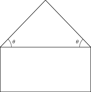
A pentagon is formed by placing an isosceles triangle on a rectangle, as shown in the diagram. If the perimeter of the pentagon is $10$ in., find the lengths of the sides of the pentagon that will maximize the area of the pentagon.

A rectangle with an isosceles triangle on top. The side of the isosceles triangle with the two equal angles of size θ overlaps the top length of the rectangle.

A rectangular box without a top (a topless box) is to be made from $12$ ft² of cardboard. Find the maximum volume of such a box.

The maximum volume is $4$ ft³. The dimensions are $1 \times 2 \times 2$ ft.

Find the minimum and maximum distances between the ellipse $x^{2} + x y + 2 y^{2} = 1$ and the origin.

Find the point on the surface $x^{2} - 2 x y + y^{2} - x + y = 0$ closest to the point $(1, 2, −3) .$

The point on the surface $x^{2} - 2 x y + y^{2} - x + y = 0$ closest to the point $(1, 2, - 3)$ is $(\frac{3}{2}, \frac{3}{2}, −3)$ .

Show that, of all the triangles inscribed in a circle of radius $R$ (see diagram), the equilateral triangle has the largest perimeter.

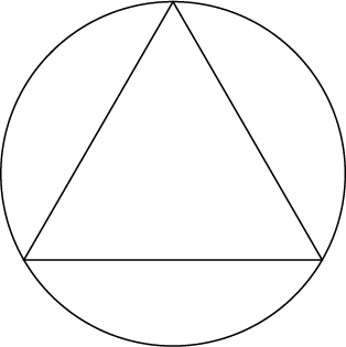
A circle with an equilateral triangle drawn inside of it such that each vertex of the triangle touches the circle.

Find the minimum distance from point $(0, 1)$ to the parabola $x^{2} = 4 y .$

$1.0$

Find the minimum distance from the parabola $y = x^{2}$ to point $(0, 3) .$

Find the minimum distance from the plane $x + y + z = 1$ to point $(2, 1, 1) .$

$\sqrt{3}$

A large container in the shape of a rectangular solid must have a volume of $480$ m³. The bottom of the container costs $5/m² to construct whereas the top and sides cost $3/m² to construct. Use Lagrange multipliers to find the dimensions of the container of this size that has the minimum cost.

Find the point on the line $y = 2 x + 3$ that is closest to point $(4, 2) .$

$(\frac{2}{5}, \frac{19}{5})$

Find the point on the plane $4 x + 3 y + z = 2$ that is closest to the point $(1, −1, 1) .$

Find the maximum value of $f (x, y) = sin x sin y,$ where $x and y$ denote the acute angles of a right triangle. Draw the contours of the function using a CAS.

$\frac{1}{2}$

An alternating series of hills and holes of amplitude 1 across xyz space.

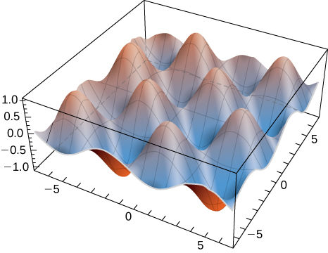
A rectangular solid is contained within a tetrahedron with vertices at

$(1, 0, 0), (0, 1, 0), (0, 0, 1),$ and the origin. The base of the box has dimensions $x, y,$ and the height of the box is $z .$ If the sum of $x, y, and z$ is 1.0, find the dimensions that maximizes the volume of the rectangular solid.

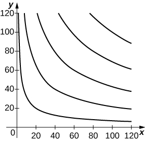
[T] By investing x units of labor and y units of capital, a watch manufacturer can produce $P (x, y) = 50 x^{0.4} y^{0.6}$ watches. Find the maximum number of watches that can be produced on a budget of $$ 20,000$ if labor costs $100/unit and capital costs $200/unit. Use a CAS to sketch a contour plot of the function.

Roughly 3365 watches at the critical point $(80, 60)$

A series of curves in the first quadrant, with the first starting near (2, 120), decreasing sharply to near (20, 20), and then decreasing slowly to (120, 5). The next curve starts near (10, 120), decreases sharply to near (40, 40), and then decreases slowly to (120, 20). The next curve starts near (20, 120), decreases sharply to near (60, 60), and then decreases slowly to (120, 40). The next curve starts near (40, 120), decreases to near (80, 80), and then decreases a little slowly to (120, 60). The last curve starts near (60, 120) and decreases rather evenly through (100, 100) to (120, 90).

Chapter Review Exercises

For the following exercises, determine whether the statement is true or false. Justify your answer with a proof or a counterexample.

The domain of $f (x, y) = x^{3} {sin}^{−1} (y)$ is $x =$ all real numbers, and $− π \leq y \leq π .$

If the function $f (x, y)$ and all its second derivatives are continuous everywhere, then $f_{x y} = f_{y x} .$

True, by Clairaut’s theorem

The linear approximation to the function of $f (x, y) = 5 x^{2} + x tan (y)$ at $(2, π)$ is given by $L (x, y) = 22 + 21 (x - 2) + (y - π) .$

$(\frac{3}{4}, \frac{9}{16})$ is a critical point of $g (x, y) = 4 x^{3} - 2 x^{2} y + y^{2} - 2 .$

False

For the following exercises, sketch the function in one graph and, in a second, sketch several level curves.

$f (x, y) = e^{− (x^{2} + 2 y^{2})} .$

$f (x, y) = x + 4 y^{2} .$

Answers may vary

For the following exercises, evaluate the following limits, if they exist. If they do not exist, prove it.

$lim_{(x, y) \to (1, 1)} \frac{4 x y}{x - 2 y^{2}}$

$lim_{(x, y) \to (0, 0)} \frac{4 x y}{x - 2 y^{2}}$

Does not exist

For the following exercises, find the largest region of continuity for the function.

$f (x, y) = x^{3} {sin}^{−1} (y)$

$g (x, y) = ln (4 - x^{2} - y^{2})$

Continuous at all points on the $x, y -plane,$ except where $x^{2} + y^{2} > 4 .$

For the following exercises, find all first derivatives, full or partial, as appropriate.

$f (x, y) = \sqrt{x^{2} - y^{2}}$

$u (x, y) = x^{4} - 3 x y + 1, x = 2 t, y = t^{3}$

$\frac{\partial u}{\partial x} = 4 x^{3} - 3 y, \frac{\partial u}{\partial y} = −3 x, \frac{d x}{d t} = 2, \frac{d y}{d t} = 3 t^{2}, \frac{d u}{d t} = 40 t^{3}$

For the following exercises, find all second partial derivatives.

$g (t, x) = 3 t^{2} - sin (x + t)$

$h (x, y, z) = \frac{x^{3} e^{2 y}}{z}$

$h_{x x} (x, y, z) = \frac{6 x e^{2 y}}{z},$ $h_{x y} (x, y, z) = \frac{6 x^{2} e^{2 y}}{z},$ $h_{x z} (x, y, z) = - \frac{3 x^{2} e^{2 y}}{z^{2}},$ $h_{y x} (x, y, z) = \frac{6 x^{2} e^{2 y}}{z},$ $h_{y y} (x, y, z) = \frac{4 x^{3} e^{2 y}}{z},$ $h_{y z} (x, y, z) = - \frac{2 x^{3} e^{2 y}}{z^{2}},$ $h_{z x} (x, y, z) = - \frac{3 x^{2} e^{2 y}}{z^{2}},$ $h_{z y} (x, y, z) = - \frac{2 x^{3} e^{2 y}}{z^{2}},$ $h_{z z} (x, y, z) = \frac{2 x^{3} e^{2 y}}{z^{3}}$

For the following exercises, find an equation of the tangent plane to the specified surface at the given point.

$z = x^{3} - 2 y^{2} + y - 1$ at point $(1, 1, −1)$

$z = e^{x} + \frac{2}{y}$ at point $(0, 1, 3)$

$z = x - 2 y + 5$

Approximate $f (x, y) = e^{x^{2}} + \sqrt{y}$ at $(0.1, 9.1) .$ Write down your linear approximation function $L (x, y) .$ How accurate is the approximation to the exact answer, rounded to four digits?

Find the differential $d z$ of $h (x, y) = 4 x^{2} + 2 x y - 3 y$ and approximate $Δ z$ at the point $(1, −2) .$ Let $Δ x = 0.1$ and $Δ y = 0.01 .$

$d z = 4 d x - d y,$ $d z (0.1, 0.01) = 0.39,$ $Δ z = 0.432$

Find the directional derivative of $f (x, y) = x^{2} + 6 x y - y^{2}$ in the direction $v = i + 4 j .$

Find the maximal directional derivative magnitude and direction for the function $f (x, y) = x^{3} + 2 x y - cos (π y)$ at point $(3, 0) .$

$3 \sqrt{85}, 〈 27, 6 〉$

For the following exercises, find the gradient.

$c (x, t) = e {(t - x)}^{2} + 3 cos (t)$

$f (x, y) = \frac{\sqrt{x} + y^{2}}{x y}$

$\nabla f (x, y) = - \frac{\sqrt{x} + 2 y^{2}}{2 x^{2} y} i + (\frac{1}{x} - \frac{1}{\sqrt{x} y^{2}}) j$

For the following exercises, find and classify the critical points.

$z = x^{3} - x y + y^{2} - 1$

For the following exercises, use Lagrange multipliers to find the maximum and minimum values for the functions with the given constraints.

$f (x, y) = x^{2} y, x^{2} + y^{2} = 4$

maximum: $\frac{16}{3 \sqrt{3}},$ minimum: $- \frac{16}{3 \sqrt{3}}$

$f (x, y) = x^{2} - y^{2}, x + 6 y = 4$

A machinist is constructing a right circular cone out of a block of aluminum. The machine gives an error of $5 %$ in height and $2 %$ in radius. Find the maximum error in the volume of the cone if the machinist creates a cone of height $6$ cm and radius $2$ cm.

$2.3228$ cm³

A trash compactor is in the shape of a cuboid. Assume the trash compactor is filled with incompressible liquid. The length and width are decreasing at rates of $2$ ft/sec and $3$ ft/sec, respectively. Find the rate at which the liquid level is rising when the length is $14$ ft, the width is $10$ ft, and the height is $4$ ft.

Glossary

constraint: an inequality or equation involving one or more variables that is used in an optimization problem; the constraint enforces a limit on the possible solutions for the problem
Lagrange multiplier: the constant (or constants) used in the method of Lagrange multipliers; in the case of one constant, it is represented by the variable $λ$
method of Lagrange multipliers: a method of solving an optimization problem subject to one or more constraints
objective function: the function that is to be maximized or minimized in an optimization problem
optimization problem: calculation of a maximum or minimum value of a function of several variables, often using Lagrange multipliers