- Write the general equation of a vector-valued function in component form and unit-vector form.
- Recognize parametric equations for a space curve.
- Describe the shape of a helix and write its equation.
- Define the limit of a vector-valued function.
Our study of vector-valued functions combines ideas from our earlier examination of single-variable calculus with our description of vectors in three dimensions from the preceding chapter. In this section we extend concepts from earlier chapters and also examine new ideas concerning curves in three-dimensional space. These definitions and theorems support the presentation of material in the rest of this chapter and also in the remaining chapters of the text.
Definition of a Vector-Valued Function
Our first step in studying the calculus of vector-valued functions is to define what exactly a vector-valued function is. We can then look at graphs of vector-valued functions and see how they define curves in both two and three dimensions.
A vector-valued function is a function of the form
where the component functions f, g, and h, are real-valued functions of the parameter t. Vector-valued functions are also written in the form
In both cases, the first form of the function defines a two-dimensional vector-valued function; the second form describes a three-dimensional vector-valued function.
The parameter t can lie between two real numbers: Another possibility is that the value of t might take on all real numbers. Last, the component functions themselves may have domain restrictions that enforce restrictions on the value of t. We often use t as a parameter because t can represent time.
For each of the following vector-valued functions, evaluate Do any of these functions have domain restrictions?
- To calculate each of the function values, substitute the appropriate value of t into the function:
To determine whether this function has any domain restrictions, consider the component functions separately. The first component function is and the second component function is Neither of these functions has a domain restriction, so the domain of is all real numbers. - To calculate each of the function values, substitute the appropriate value of t into the function:
To determine whether this function has any domain restrictions, consider the component functions separately. The first component function is the second component function is and the third component function is The first two functions are not defined for odd multiples of so the function is not defined for odd multiples of Therefore, where n is any integer.
For the vector-valued function evaluate Does this function have any domain restrictions?
The domain of is all real numbers.
Example 3.1 illustrates an important concept. The domain of a vector-valued function consists of real numbers. The domain can be all real numbers or a subset of the real numbers. The range of a vector-valued function consists of vectors. Each real number in the domain of a vector-valued function is mapped to either a two- or a three-dimensional vector.
Graphing Vector-Valued Functions
Recall that a plane vector consists of two quantities: direction and magnitude. Given any point in the plane (the initial point), if we move in a specific direction for a specific distance, we arrive at a second point. This represents the terminal point of the vector. We calculate the components of the vector by subtracting the coordinates of the initial point from the coordinates of the terminal point.
A vector is considered to be in standard position if the initial point is located at the origin. When graphing a vector-valued function, we typically graph the vectors in the domain of the function in standard position, because doing so guarantees the uniqueness of the graph. This convention applies to the graphs of three-dimensional vector-valued functions as well. The graph of a vector-valued function of the form consists of the set of all and the path it traces is called a plane curve. The graph of a vector-valued function of the form consists of the set of all and the path it traces is called a space curve. Any representation of a plane curve or space curve using a vector-valued function is called a vector parameterization of the curve.
Create a graph of each of the following vector-valued functions:
- The plane curve represented by
- The plane curve represented by
- The space curve represented by
- As with any graph, we start with a table of values. We then graph each of the vectors in the second column of the table in standard position and connect the terminal points of each vector to form a curve (Figure 3.2). This curve turns out to be an ellipse centered at the origin.
Table 3.1 Table of Values for t t 0 This is a table with two columns. The first column is labeled with “t”. The second column is labeled with the function “r(t)”. There are 9 rows in the table. The first row contains the entries 0 and 4i for the first and the second column. The second row contains the entries pi/4 and 2(the square root of 2)i + 2(the square root of 3)/2 j. The third row contains the entries pi/2 and 3j. The fourth row contains the entries 3pi/4 and -2(the square root of 2)i + 2(the square root of 3)/2 j. The fifth row contains the entries pi and -4i. The sixth row contains the entries 5pi/4 and -2(the square root of 2)i - 2(the square root of 3)/2 j. The seventh row contains the entries 3pi/2 and -3j. The eighth row contains the entries 7pi/4 and 2(the square root of 2)i - 2(the square root of 3)/2 j. The ninth row contains the entries 2pi and 4i.
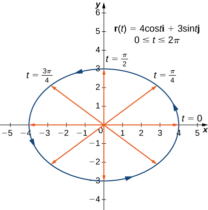
Figure 3.2 The graph of the first vector-valued function is an ellipse. - The table of values for is as follows:
Table 3.2 Table of Values for t t 0 This is a table with two columns. The first column is labeled with “t”. The second column is labeled with the function “r(t)”. There are 9 rows in the table. The first row contains the entries 0 and 4i for the first and the second column. The second row contains the entries pi/4 and 2(the square root of 2)i + 2(the square root of 3)/2 j. The third row contains the entries pi/2 and 3j. The fourth row contains the entries 3pi/4 and -2(the square root of 2)i + 2(the square root of 3)/2 j. The fifth row contains the entries pi and -4i. The sixth row contains the entries 5pi/4 and -2(the square root of 2)i - 2(the square root of 3)/2 j. The seventh row contains the entries 3pi/2 and -3j. The eighth row contains the entries 7pi/4 and 2(the square root of 2)i - 2(the square root of 3)/2 j. The ninth row contains the entries 2pi and 4i.
The graph of this curve is also an ellipse centered at the origin.
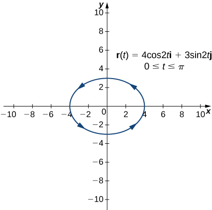
Figure 3.3 The graph of the second vector-valued function is also an ellipse. - We go through the same procedure for a three-dimensional vector function.
Table 3.3 Table of Values for t t 0 This is a table with two columns. The first column is labeled with “t”. The second column is labeled with the function “r(t)”. There are 9 rows in the table. The first row contains the entries 0 and 4i for the first and the second column. The second row contains the entries pi/4 and 2(the square root of 2)i + 2(the square root of 3)/2 j + pi/4 k. The third row contains the entries pi/2 and 3j + pi/2k. The fourth row contains the entries 3pi/4 and -2(the square root of 2)i + 2(the square root of 3)/2 j + 3pi/4 k. The fifth row contains the entries pi and -4i + pik. The sixth row contains the entries 5pi/4 and -2(the square root of 2)i - 2(the square root of 3)/2 j + 5pi/4 k. The seventh row contains the entries 3pi/2 and -3j + 3pi/2 k. The eighth row contains the entries 7pi/4 and 2(the square root of 2)i - 2(the square root of 3)/2 j + 7pi/4 k. The ninth row contains the entries 2pi and 4i +2pik.
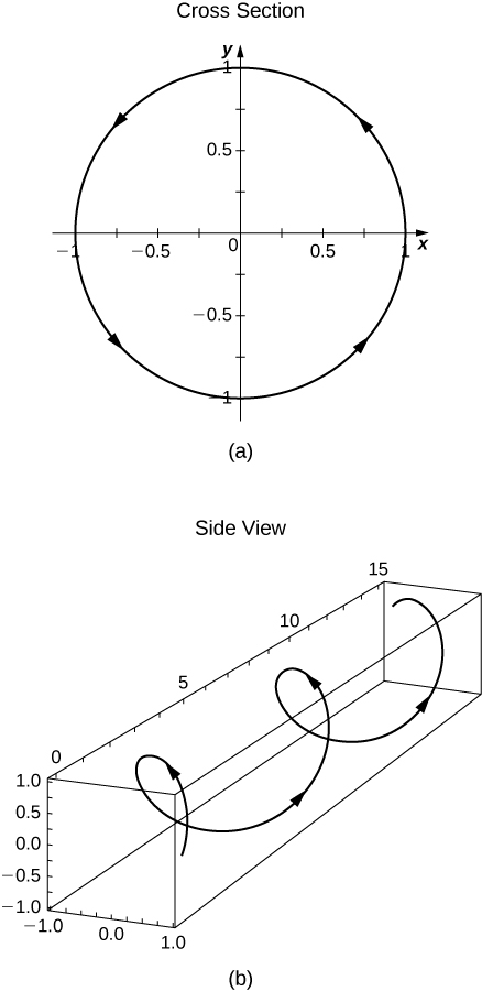
The values then repeat themselves, except for the fact that the coefficient of k is always increasing (Figure 3.4). This curve is called a helix. Notice that if the k component is eliminated, then the function becomes which is a unit circle centered at the origin.
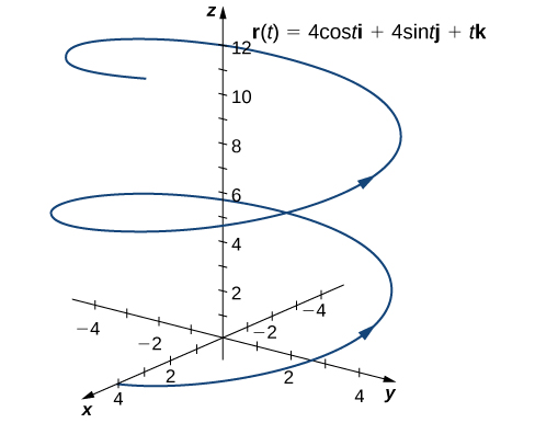
Figure 3.4 The graph of the third vector-valued function is a helix.
You may notice that the graphs in parts a. and b. are identical. This happens because the function describing curve b is a so-called reparameterization of the function describing curve a. In fact, any curve has an infinite number of reparameterizations; for example, we can replace t with in any of the three previous curves without changing the shape of the curve. The interval over which t is defined may change, but that is all. We return to this idea later in this chapter when we study arc-length parameterization.
As mentioned, the name of the shape of the curve of the graph in Example 3.2c. is a helix (Figure 3.4). The curve resembles a spring, with a circular cross-section looking down along the z-axis. It is possible for a helix to be elliptical in cross-section as well. For example, the vector-valued function describes an elliptical helix. The projection of this helix into the is an ellipse. Last, the arrows in the graph of this helix indicate the orientation of the curve as t progresses from 0 to
Create a graph of the vector-valued function
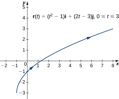
Start by making a table of values, then graph the vectors for each value of t.
At this point, you may notice a similarity between vector-valued functions and parameterized curves. Indeed, given a vector-valued function we can define and If a restriction exists on the values of t (for example, t is restricted to the interval for some constants then this restriction is enforced on the parameter. The graph of the parameterized function would then agree with the graph of the vector-valued function, except that the vector-valued graph would represent vectors rather than points. Since we can parameterize a curve defined by a function it is also possible to represent an arbitrary plane curve by a vector-valued function.
Limits and Continuity of a Vector-Valued Function
We now take a look at the limit of a vector-valued function. This is important to understand to study the calculus of vector-valued functions.
A vector-valued function r approaches the limit L as t approaches a, written
provided
This is a rigorous definition of the limit of a vector-valued function. In practice, we use the following theorem:
Let f, g, and h be functions of t. Then the limit of the vector-valued function as t approaches a is given by
provided the limits exist. Similarly, the limit of the vector-valued function as t approaches a is given by
provided the limits exist.
In the following example, we show how to calculate the limit of a vector-valued function.
For each of the following vector-valued functions, calculate for
- Use Equation 3.3 and substitute the value into the two component expressions:
- Use Equation 3.4 and substitute the value into the three component expressions:
Now that we know how to calculate the limit of a vector-valued function, we can define continuity at a point for such a function.
Let f, g, and h be functions of t. Then, the vector-valued function is continuous at point if the following three conditions hold:
- exists
- exists
Similarly, the vector-valued function is continuous at point if the following three conditions hold:
- exists
- exists
Key Concepts
- A vector-valued function is a function of the form or where the component functions f, g, and h are real-valued functions of the parameter t.
- The graph of a vector-valued function of the form is called a plane curve. The graph of a vector-valued function of the form is called a space curve.
- It is possible to represent an arbitrary plane curve by a vector-valued function.
- To calculate the limit of a vector-valued function, calculate the limits of the component functions separately.
Key Equations
| Vector-valued function | |
| Limit of a vector-valued function |
.
Give the component functions and for the vector-valued function
Given find the following values (if possible).
Sketch the curve of the vector-valued function and give the orientation of the curve. Sketch asymptotes as a guide to the graph.
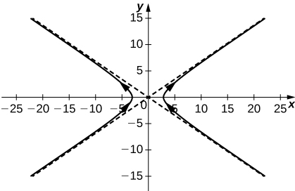
Evaluate
Given the vector-valued function find the following values:
- Is continuous at
- Graph
a. b. c. Yes, the limit as t approaches is equal to d.
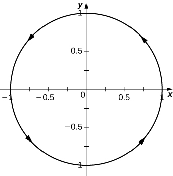
Given the vector-valued function find the following values:
- Is continuous at
Let Find the following values:
- Is continuous at
a. b. c. Yes
Find the limit of the following vector-valued functions at the indicated value of t.
for
for
The limit does not exist because the limit of as t approaches infinity does not exist.
Describe the curve defined by the vector-valued function
Find the domain of the vector-valued functions.
Domain:
where k is an integer
Domain:
Domain:
where n is an integer
Let and use it to answer the following questions.
For what values of t is continuous?
Sketch the graph of
Find the domain of
For what values of t is continuous?
All t such that
Eliminate the parameter t, write the equation in Cartesian coordinates, then sketch the graphs of the vector-valued functions.
(Hint: Let and Solve the first equation for x in terms of t and substitute this result into the second equation.)
a variation of the cube-root function
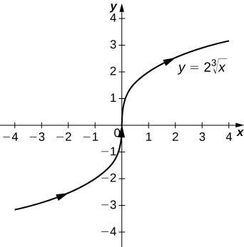
a circle centered at with radius 3, and a counterclockwise orientation
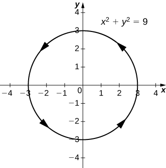
Use a graphing utility to sketch each of the following vector-valued functions:
[T]
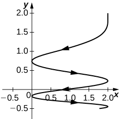
[T]
[T]
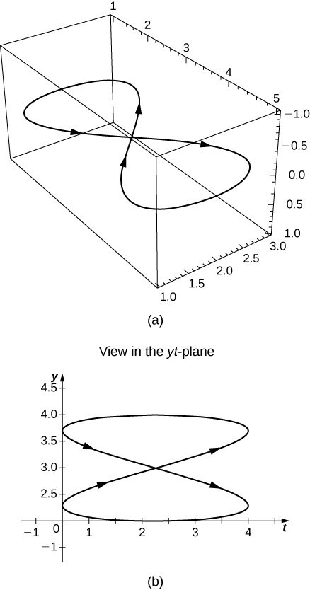
Find a vector-valued function that traces out the given curve in the indicated direction.
clockwise and counterclockwise
from left to right
For left to right, where t increases
The line through P and Q where P is and Q is
Consider the curve described by the vector-valued function
What is the initial point of the path corresponding to
What is
[T] Use technology to sketch the curve.
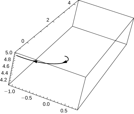
Eliminate the parameter t to show that where
[T] Let Use technology to graph the curve (called the roller-coaster curve) over the interval Choose at least two views to determine the peaks and valleys.
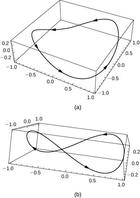
[T] Use the result of the preceding problem to construct an equation of a roller coaster with a steep drop from the peak and steep incline from the “valley.” Then, use technology to graph the equation.
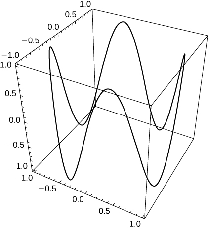
Use the results of the preceding two problems to construct an equation of a path of a roller coaster with more than two turning points (peaks and valleys).
One possibility is By increasing the coefficient of t in the third component, the number of turning points will increase.
- Graph the curve using two viewing angles of your choice to see the overall shape of the curve.
- Does the curve resemble a “slinky”?
- What changes to the equation should be made to increase the number of coils of the slinky?
Glossary
- component functions
- the component functions of the vector-valued function are and and the component functions of the vector-valued function are and
- helix
- a three-dimensional curve in the shape of a spiral
- limit of a vector-valued function
- a vector-valued function has a limit L as t approaches a if
- plane curve
- the set of ordered pairs together with their defining parametric equations and
- reparameterization
- an alternative parameterization of a given vector-valued function
- space curve
- the set of ordered triples together with their defining parametric equations and
- vector parameterization
- any representation of a plane or space curve using a vector-valued function
- vector-valued function
- a function of the form or where the component functions f, g, and h are real-valued functions of the parameter t
Substitute the appropriate values of t into the function.