6.4 Working with Taylor Series

Write the terms of the binomial series.
Recognize the Taylor series expansions of common functions.
Recognize and apply techniques to find the Taylor series for a function.
Use Taylor series to solve differential equations.
Use Taylor series to evaluate nonelementary integrals.

In the preceding section, we defined Taylor series and showed how to find the Taylor series for several common functions by explicitly calculating the coefficients of the Taylor polynomials. In this section we show how to use those Taylor series to derive Taylor series for other functions. We then present two common applications of power series. First, we show how power series can be used to solve differential equations. Second, we show how power series can be used to evaluate integrals when the antiderivative of the integrand cannot be expressed in terms of elementary functions. In one example, we consider $\int e^{− x^{2}} d x,$ an integral that arises frequently in probability theory.

The Binomial Series

Our first goal in this section is to determine the Maclaurin series for the function $f (x) = {(1 + x)}^{r}$ for all real numbers $r .$ The Maclaurin series for this function is known as the binomial series. We begin by considering the simplest case: $r$ is a nonnegative integer. We recall that, for $r = 0, 1, 2, 3, 4, f (x) = {(1 + x)}^{r}$ can be written as

\begin{matrix} f (x) = {(1 + x)}^{0} = 1, \\ f (x) = {(1 + x)}^{1} = 1 + x, \\ f (x) = {(1 + x)}^{2} = 1 + 2 x + x^{2}, \\ f (x) = {(1 + x)}^{3} = 1 + 3 x + 3 x^{2} + x^{3}, \\ f (x) = {(1 + x)}^{4} = 1 + 4 x + 6 x^{2} + 4 x^{3} + x^{4} . \end{matrix}

The expressions on the right-hand side are known as binomial expansions and the coefficients are known as binomial coefficients. More generally, for any nonnegative integer $r,$ the binomial coefficient of $x^{n}$ in the binomial expansion of ${(1 + x)}^{r}$ is given by

(\begin{matrix} r \\ n \end{matrix}) = \frac{r!}{n! (r - n)!}

6.6

and

\begin{matrix} f (x) & = {(1 + x)}^{r} \\ = (\begin{matrix} r \\ 0 \end{matrix}) 1 + (\begin{matrix} r \\ 1 \end{matrix}) x + (\begin{matrix} r \\ 2 \end{matrix}) x^{2} + (\begin{matrix} r \\ 3 \end{matrix}) x^{3} + ⋯ + (\begin{matrix} r \\ r - 1 \end{matrix}) x^{r - 1} + (\begin{matrix} r \\ r \end{matrix}) x^{r} \\ = \sum_{n = 0}^{r} (\begin{matrix} r \\ n \end{matrix}) x^{n} . \end{matrix}

6.7

For example, using this formula for $r = 5,$ we see that

\begin{matrix} f (x) & = {(1 + x)}^{5} \\ = (\begin{matrix} 5 \\ 0 \end{matrix}) 1 + (\begin{matrix} 5 \\ 1 \end{matrix}) x + (\begin{matrix} 5 \\ 2 \end{matrix}) x^{2} + (\begin{matrix} 5 \\ 3 \end{matrix}) x^{3} + (\begin{matrix} 5 \\ 4 \end{matrix}) x^{4} + (\begin{matrix} 5 \\ 5 \end{matrix}) x^{5} \\ = \frac{5!}{0! 5!} 1 + \frac{5!}{1! 4!} x + \frac{5!}{2! 3!} x^{2} + \frac{5!}{3! 2!} x^{3} + \frac{5!}{4! 1!} x^{4} + \frac{5!}{5! 0!} x^{5} \\ = 1 + 5 x + 10 x^{2} + 10 x^{3} + 5 x^{4} + x^{5} . \end{matrix}

We now consider the case when the exponent $r$ is any real number, not necessarily a nonnegative integer. If $r$ is not a nonnegative integer, then $f (x) = {(1 + x)}^{r}$ cannot be written as a finite polynomial. However, we can find a power series for $f .$ Specifically, we look for the Maclaurin series for $f .$ To do this, we find the derivatives of $f$ and evaluate them at $x = 0 .$

\begin{matrix} f (x) & = & {(1 + x)}^{r} & f (0) & = & 1 \\ f^{'} (x) & = & r {(1 + x)}^{r - 1} & f' (0) & = & r \\ f^{″} (x) & = & r (r - 1) {(1 + x)}^{r - 2} & f^{″} (0) & = & r (r - 1) \\ f ‴ (x) & = & r (r - 1) (r - 2) {(1 + x)}^{r - 3} & f ‴ (0) & = & r (r - 1) (r - 2) \\ f^{(n)} (x) & = & r (r - 1) (r - 2) ⋯ (r - n + 1) {(1 + x)}^{r - n} & f^{(n)} (0) & = & r (r - 1) (r - 2) ⋯ (r - n + 1) \end{matrix}

We conclude that the coefficients in the binomial series are given by

\frac{f^{(n)} (0)}{n!} = \frac{r (r - 1) (r - 2) ⋯ (r - n + 1)}{n!} .

6.8

We note that if $r$ is a nonnegative integer, then the $(r + 1) st$ derivative $f^{(r + 1)}$ is the zero function, and the series terminates. In addition, if $r$ is a nonnegative integer, then Equation 6.8 for the coefficients agrees with Equation 6.6 for the coefficients, and the formula for the binomial series agrees with Equation 6.7 for the finite binomial expansion. More generally, to denote the binomial coefficients for any real number $r,$ we define

(\begin{matrix} r \\ n \end{matrix}) = \frac{r (r - 1) (r - 2) ⋯ (r - n + 1)}{n!} .

With this notation, we can write the binomial series for ${(1 + x)}^{r}$ as

\sum_{n = 0}^{\infty} (\begin{matrix} r \\ n \end{matrix}) x^{n} = 1 + r x + \frac{r (r - 1)}{2!} x^{2} + ⋯ + \frac{r (r - 1) ⋯ (r - n + 1)}{n!} x^{n} + ⋯ .

6.9

We now need to determine the interval of convergence for the binomial series Equation 6.9. We apply the ratio test. Consequently, we consider

\begin{matrix} \frac{| a_{n + 1} |}{| a_{n} |} & = \frac{{| r (r - 1) (r - 2) ⋯ (r - n) | x | |}^{n + 1}}{(n + 1)!} \cdot \frac{n!}{| r (r - 1) (r - 2) ⋯ (r - n + 1) | {| x |}^{n}} \\ = \frac{| r - n | | x |}{| n + 1 |} . \end{matrix}

Since

lim_{n \to \infty} \frac{| a_{n + 1} |}{| a_{n} |} = | x | < 1

if and only if $| x | < 1,$ we conclude that the interval of convergence for the binomial series is $(−1, 1) .$ The behavior at the endpoints depends on $r .$ It can be shown that for $r \geq 0$ the series converges at both endpoints; for $−1 < r < 0,$ the series converges at $x = 1$ and diverges at $x = −1;$ and for $r < −1,$ the series diverges at both endpoints. The binomial series does converge to ${(1 + x)}^{r}$ in $(−1, 1)$ for all real numbers $r,$ but proving this fact by showing that the remainder $R_{n} (x) \to 0$ is difficult.

Definition

For any real number $r,$ the Maclaurin series for $f (x) = {(1 + x)}^{r}$ is the binomial series. It converges to $f$ for $| x | < 1,$ and we write

\begin{matrix} {(1 + x)}^{r} & = \sum_{n = 0}^{\infty} (\begin{matrix} r \\ n \end{matrix}) x^{n} \\ = 1 + r x + \frac{r (r - 1)}{2!} x^{2} + ⋯ + \frac{r (r - 1) ⋯ (r - n + 1)}{n!} x^{n} + ⋯ \end{matrix}

for $| x | < 1 .$

We can use this definition to find the binomial series for $f (x) = \sqrt{1 + x}$ and use the series to approximate $\sqrt{1.5} .$

Finding Binomial Series

Find the binomial series for $f (x) = \sqrt{1 + x} .$
Use the third-order Maclaurin polynomial $p_{3} (x)$ to estimate $\sqrt{1.5} .$ Use Taylor’s theorem to bound the error. Use a graphing utility to compare the graphs of $f$ and $p_{3} .$

Here $r = \frac{1}{2} .$ Using the definition for the binomial series, we obtain

$\begin{matrix} \sqrt{1 + x} & = 1 + \frac{1}{2} x + \frac{(1 / 2) (− 1 / 2)}{2!} x^{2} + \frac{(1 / 2) (− 1 / 2) (− 3 / 2)}{3!} x^{3} + ⋯ \\ = 1 + \frac{1}{2} x - \frac{1}{2!} \frac{1}{2^{2}} x^{2} + \frac{1}{3!} \frac{1 \cdot 3}{2^{3}} x^{3} - ⋯ + \frac{{(−1)}^{n + 1}}{n!} \frac{1 \cdot 3 \cdot 5 ⋯ (2 n - 3)}{2^{n}} x^{n} + ⋯ \\ = 1 + \sum_{n = 1}^{\infty} \frac{{(−1)}^{n + 1}}{n!} \frac{1 \cdot 3 \cdot 5 ⋯ (2 n - 3)}{2^{n}} x^{n} . \end{matrix}$
From the result in part a. the third-order Maclaurin polynomial is

$p_{3} (x) = 1 + \frac{1}{2} x - \frac{1}{8} x^{2} + \frac{1}{16} x^{3} .$

Therefore,

$\begin{matrix} \sqrt{1.5} & = \sqrt{1 + 0.5} \\ \approx 1 + \frac{1}{2} (0.5) - \frac{1}{8} {(0.5)}^{2} + \frac{1}{16} {(0.5)}^{3} \\ \approx 1.2266. \end{matrix}$

From Taylor’s theorem, the error satisfies

$R_{3} (0.5) = \frac{f^{(4)} (c)}{4!} {(0.5)}^{4}$

for some $c$ between $0$ and $0.5 .$ Since $f^{(4)} (x) = - \frac{15}{2^{4} {(1 + x)}^{7 / 2}},$ and the maximum value of $| f^{(4)} (x) |$ on the interval $(0, 0.5)$ occurs at $x = 0,$ we have

$| R_{3} (0.5) | \leq \frac{15}{4! 2^{4}} {(0.5)}^{4} \approx 0.00244 .$

The function and the Maclaurin polynomial $p_{3}$ are graphed in Figure 6.10.

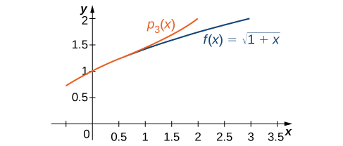
Figure 6.10 The third-order Maclaurin polynomial $p_{3} (x)$ provides a good approximation for $f (x) = \sqrt{1 + x}$ for $x$ near zero.

Find the binomial series for $f (x) = \frac{1}{{(1 + x)}^{2}} .$

$\sum_{n = 0}^{\infty} {(−1)}^{n} (n + 1) x^{n}$

Hint

Use the definition of binomial series for $r = −2 .$

Common Functions Expressed as Taylor Series

At this point, we have derived Maclaurin series for exponential, trigonometric, and logarithmic functions, as well as functions of the form $f (x) = {(1 + x)}^{r} .$ In Table 6.1, we summarize the results of these series. We remark that the convergence of the Maclaurin series for $f (x) = ln (1 + x)$ at the endpoint $x = 1$ and the Maclaurin series for $f (x) = {tan}^{−1} x$ at the endpoints $x = 1$ and $x = −1$ relies on a more advanced theorem than we present here. (Refer to Abel’s theorem for a discussion of this more technical point.)

Table 6.1 Maclaurin Series for Common Functions
Function	Maclaurin Series	Interval of Convergence
$f (x) = \frac{1}{1 - x}$	$\sum_{n = 0}^{\infty} x^{n}$	$−1 < x < 1$
$f (x) = e^{x}$	$\sum_{n = 0}^{\infty} \frac{x^{n}}{n!}$	$− \infty < x < \infty$
$f (x) = sin x$	$\sum_{n = 0}^{\infty} {(−1)}^{n} \frac{x^{2 n + 1}}{(2 n + 1)!}$	$− \infty < x < \infty$
$f (x) = cos x$	$\sum_{n = 0}^{\infty} {(−1)}^{n} \frac{x^{2 n}}{(2 n)!}$	$− \infty < x < \infty$
$f (x) = ln (1 + x)$	$\sum_{n = 1}^{\infty} {(−1)}^{n + 1} \frac{x^{n}}{n}$	$−1 < x \leq 1$
$f (x) = {tan}^{−1} x$	$\sum_{n = 0}^{\infty} {(−1)}^{n} \frac{x^{2 n + 1}}{2 n + 1}$	$−1 \leq x \leq 1$
$f (x) = {(1 + x)}^{r}$	$\sum_{n = 0}^{\infty} (\begin{matrix} r \\ n \end{matrix}) x^{n}$	$−1 < x < 1$

Earlier in the chapter, we showed how you could combine power series to create new power series. Here we use these properties, combined with the Maclaurin series in Table 6.1, to create Maclaurin series for other functions.

Deriving Maclaurin Series from Known Series

Find the Maclaurin series of each of the following functions by using one of the series listed in Table 6.1.

$f (x) = cos \sqrt{x}$
$f (x) = sinh x$

Using the Maclaurin series for $cos x$ we find that the Maclaurin series for $cos \sqrt{x}$ is given by

$\begin{matrix} \sum_{n = 0}^{\infty} \frac{{(−1)}^{n} {(\sqrt{x})}^{2 n}}{(2 n)!} & = \sum_{n = 0}^{\infty} \frac{{(−1)}^{n} x^{n}}{(2 n)!} \\ = 1 - \frac{x}{2!} + \frac{x^{2}}{4!} - \frac{x^{3}}{6!} + \frac{x^{4}}{8!} - ⋯ . \end{matrix}$

This series converges to $cos \sqrt{x}$ for all $x$ in the domain of $cos \sqrt{x};$ that is, for all $x \geq 0 .$
To find the Maclaurin series for $sinh x,$ we use the fact that

$sinh x = \frac{e^{x} - e^{− x}}{2} .$

Using the Maclaurin series for $e^{x},$ we see that the $n th$ term in the Maclaurin series for $sinh x$ is given by

$\frac{x^{n}}{n!} - \frac{{(− x)}^{n}}{n!} .$

For $n$ even, this term is zero. For $n$ odd, this term is $\frac{2 x^{n}}{n!} .$ Therefore, the Maclaurin series for $sinh x$ has only odd-order terms and is given by

$\sum_{n = 0}^{\infty} \frac{x^{2 n + 1}}{(2 n + 1)!} = x + \frac{x^{3}}{3!} + \frac{x^{5}}{5!} + ⋯ .$

Find the Maclaurin series for $sin (x^{2}) .$

$\sum_{n = 0}^{\infty} \frac{{(−1)}^{n} x^{4 n + 2}}{(2 n + 1)!}$

Hint

Use the Maclaurin series for $sin x .$

We also showed previously in this chapter how power series can be differentiated term by term to create a new power series. In Example 6.19, we differentiate the binomial series for $\sqrt{1 + x}$ term by term to find the binomial series for $\frac{1}{\sqrt{1 + x}} .$ Note that we could construct the binomial series for $\frac{1}{\sqrt{1 + x}}$ directly from the definition, but differentiating the binomial series for $\sqrt{1 + x}$ is an easier calculation.

Differentiating a Series to Find a New Series

Use the binomial series for $\sqrt{1 + x}$ to find the binomial series for $\frac{1}{\sqrt{1 + x}} .$

The two functions are related by

\frac{d}{d x} \sqrt{1 + x} = \frac{1}{2 \sqrt{1 + x}},

so the binomial series for $\frac{1}{\sqrt{1 + x}}$ is given by

\begin{matrix} \frac{1}{\sqrt{1 + x}} & = 2 \frac{d}{d x} \sqrt{1 + x} \\ = 1 + \sum_{n = 1}^{\infty} \frac{{(−1)}^{n}}{n!} \frac{1 \cdot 3 \cdot 5 ⋯ (2 n - 1)}{2^{n}} x^{n} . \end{matrix}

Find the binomial series for $f (x) = \frac{1}{{(1 + x)}^{3 / 2}}$

$\sum_{n = 1}^{\infty} \frac{{(−1)}^{n}}{n!} \frac{1 \cdot 3 \cdot 5 ⋯ (2 n - 1)}{2^{n}} x^{n}$

Hint

Differentiate the series for $\frac{1}{\sqrt{1 + x}} .$

In this example, we differentiated a known Taylor series to construct a Taylor series for another function. The ability to differentiate power series term by term makes them a powerful tool for solving differential equations. We now show how this is accomplished.

Solving Differential Equations with Power Series

Consider the differential equation

y^{'} (x) = y .

Recall that this is a first-order separable equation and its solution is $y = C e^{x} .$ This equation is easily solved using techniques discussed earlier in the text. For most differential equations, however, we do not yet have analytical tools to solve them. Power series are an extremely useful tool for solving many types of differential equations. In this technique, we look for a solution of the form $y = \sum_{n = 0}^{\infty} c_{n} x^{n}$ and determine what the coefficients would need to be. In the next example, we consider an initial-value problem involving $y^{'} = y$ to illustrate the technique.

Power Series Solution of a Differential Equation

Use power series to solve the initial-value problem

y^{'} = y, y (0) = 3 .

Suppose that there exists a power series solution

y (x) = \sum_{n = 0}^{\infty} c_{n} x^{n} = c_{0} + c_{1} x + c_{2} x^{2} + c_{3} x^{3} + c_{4} x^{4} + ⋯ .

Differentiating this series term by term, we obtain

y^{'} = c_{1} + 2 c_{2} x + 3 c_{3} x^{2} + 4 c_{4} x^{3} + ⋯ .

If y satisfies the differential equation, then

c_{0} + c_{1} x + c_{2} x^{2} + c_{3} x^{3} + ⋯ = c_{1} + 2 c_{2} x + 3 c_{3} x^{2} + 4 c_{3} x^{3} + ⋯ .

Using Differentiating and Integrating Power Series on the uniqueness of power series representations, we know that these series can only be equal if their coefficients are equal. Therefore,

\begin{matrix} c_{0} = c_{1}, \\ c_{1} = 2 c_{2}, \\ c_{2} = 3 c_{3}, \\ c_{3} = 4 c_{4}, \\ ⋮ . \end{matrix}

Using the initial condition $y (0) = 3$ combined with the power series representation

y (x) = c_{0} + c_{1} x + c_{2} x^{2} + c_{3} x^{3} + ⋯,

we find that $c_{0} = 3 .$ We are now ready to solve for the rest of the coefficients. Using the fact that $c_{0} = 3,$ we have

\begin{matrix} c_{1} = c_{0} = 3 = \frac{3}{1!}, \\ c_{2} = \frac{c_{1}}{2} = \frac{3}{2} = \frac{3}{2!}, \\ c_{3} = \frac{c_{2}}{3} = \frac{3}{3 \cdot 2} = \frac{3}{3!}, \\ c_{4} = \frac{c_{3}}{4} = \frac{3}{4 \cdot 3 \cdot 2} = \frac{3}{4!} . \end{matrix}

Therefore,

\begin{matrix} y & = 3 [1 + \frac{1}{1!} x + \frac{1}{2!} x^{2} + \frac{1}{3!} x^{3} + \frac{1}{4!} x^{4} + ⋯] \\ = 3 \sum_{n = 0}^{\infty} \frac{x^{n}}{n!} . \end{matrix}

You might recognize

\sum_{n = 0}^{\infty} \frac{x^{n}}{n!}

as the Taylor series for $e^{x} .$ Therefore, the solution is $y = 3 e^{x} .$

Use power series to solve $y^{'} = 2 y, y (0) = 5 .$

$y = 5 e^{2 x}$

Hint

The equations for the first several coefficients $c_{n}$ will satisfy $c_{0} = 2 c_{1}, c_{1} = 2 \cdot 2 c_{2}, c_{2} = 2 \cdot 3 c_{3},….$ In general, for all $n \geq 0, c_{n} = 2 (n + 1) C_{n + 1} .$

We now consider an example involving a differential equation that we cannot solve using previously discussed methods. This differential equation

y^{″} - x y = 0

is known as Airy’s equation. It has many applications in mathematical physics, such as modeling the diffraction of light. Here we show how to solve it using power series.

Power Series Solution of Airy’s Equation

Use power series to solve

y^{″} - x y = 0

with the initial conditions $y (0) = a$ and $y' (0) = b .$

We look for a solution of the form

y = \sum_{n = 0}^{\infty} c_{n} x^{n} = c_{0} + c_{1} x + c_{2} x^{2} + c_{3} x^{3} + c_{4} x^{4} + ⋯ .

Differentiating this function term by term, we obtain

\begin{matrix} y^{'} & = & c_{1} + 2 c_{2} x + 3 c_{3} x^{2} + 4 c_{4} x^{3} + ⋯, \\ y^{″} & = & 2 \cdot 1 c_{2} + 3 \cdot 2 c_{3} x + 4 \cdot 3 c_{4} x^{2} + ⋯ . \end{matrix}

If y satisfies the equation $y^{″} = x y,$ then

2 \cdot 1 c_{2} + 3 \cdot 2 c_{3} x + 4 \cdot 3 c_{4} x^{2} + ⋯ = x (c_{0} + c_{1} x + c_{2} x^{2} + c_{3} x^{3} + ⋯) .

Using Differentiating and Integrating Power Series on the uniqueness of power series representations, we know that coefficients of the same degree must be equal. Therefore,

\begin{matrix} 2 \cdot 1 c_{2} = 0, \\ 3 \cdot 2 c_{3} = c_{0}, \\ 4 \cdot 3 c_{4} = c_{1}, \\ 5 \cdot 4 c_{5} = c_{2}, \\ ⋮ . \end{matrix}

More generally, for $n \geq 3,$ we have $n \cdot (n - 1) c_{n} = c_{n - 3} .$ In fact, all coefficients can be written in terms of $c_{0}$ and $c_{1} .$ To see this, first note that $c_{2} = 0 .$ Then

\begin{matrix} c_{3} = \frac{c_{0}}{3 \cdot 2}, \\ c_{4} = \frac{c_{1}}{4 \cdot 3} . \end{matrix}

For $c_{5}, c_{6}, c_{7},$ we see that

\begin{matrix} c_{5} = \frac{c_{2}}{5 \cdot 4} = 0, \\ c_{6} = \frac{c_{3}}{6 \cdot 5} = \frac{c_{0}}{6 \cdot 5 \cdot 3 \cdot 2}, \\ c_{7} = \frac{c_{4}}{7 \cdot 6} = \frac{c_{1}}{7 \cdot 6 \cdot 4 \cdot 3} . \end{matrix}

Therefore, the series solution of the differential equation is given by

y = c_{0} + c_{1} x + 0 \cdot x^{2} + \frac{c_{0}}{3 \cdot 2} x^{3} + \frac{c_{1}}{4 \cdot 3} x^{4} + 0 \cdot x^{5} + \frac{c_{0}}{6 \cdot 5 \cdot 3 \cdot 2} x^{6} + \frac{c_{1}}{7 \cdot 6 \cdot 4 \cdot 3} x^{7} + ⋯ .

The initial condition $y (0) = a$ implies $c_{0} = a .$ Differentiating this series term by term and using the fact that $y^{'} (0) = b,$ we conclude that $c_{1} = b .$ Therefore, the solution of this initial-value problem is

y = a (1 + \frac{x^{3}}{3 \cdot 2} + \frac{x^{6}}{6 \cdot 5 \cdot 3 \cdot 2} + ⋯) + b (x + \frac{x^{4}}{4 \cdot 3} + \frac{x^{7}}{7 \cdot 6 \cdot 4 \cdot 3} + ⋯) .

Use power series to solve $y^{″} + x^{2} y = 0$ with the initial condition $y (0) = a$ and $y^{'} (0) = b .$

$y = a (1 - \frac{x^{4}}{3 \cdot 4} + \frac{x^{8}}{3 \cdot 4 \cdot 7 \cdot 8} - ⋯) + b (x - \frac{x^{5}}{4 \cdot 5} + \frac{x^{9}}{4 \cdot 5 \cdot 8 \cdot 9} - ⋯)$

Hint

The coefficients satisfy $c_{0} = a, c_{1} = b, c_{2} = 0, c_{3} = 0,$ and for $n \geq 4, n (n - 1) c_{n} = − c_{n - 4} .$

Evaluating Nonelementary Integrals

Solving differential equations is one common application of power series. We now turn to a second application. We show how power series can be used to evaluate integrals involving functions whose antiderivatives cannot be expressed using elementary functions.

One integral that arises often in applications in probability theory is $\int e^{− x^{2}} d x .$ Unfortunately, the antiderivative of the integrand $e^{− x^{2}}$ is not an elementary function. By elementary function, we mean a function that can be written using a finite number of algebraic combinations or compositions of exponential, logarithmic, trigonometric, or power functions. We remark that the term “elementary function” is not synonymous with noncomplicated function. For example, the function $f (x) = \sqrt{x^{2} - 3 x} + e^{x^{3}} - sin (5 x + 4)$ is an elementary function, although not a particularly simple-looking function. Any integral of the form $\int f (x) d x$ where the antiderivative of $f$ cannot be written as an elementary function is considered a nonelementary integral.

Nonelementary integrals cannot be evaluated using the basic integration techniques discussed earlier. One way to evaluate such integrals is by expressing the integrand as a power series and integrating term by term. We demonstrate this technique by considering $\int e^{− x^{2}} d x .$

Using Taylor Series to Evaluate a Definite Integral

Express $\int e^{− x^{2}} d x$ as an infinite series.
Evaluate $\int_{0}^{1} e^{− x^{2}} d x$ to within an error of $0.01 .$

The Maclaurin series for $e^{− x^{2}}$ is given by

$\begin{matrix} e^{− x^{2}} & = \sum_{n = 0}^{\infty} \frac{{(− x^{2})}^{n}}{n!} \\ = 1 - x^{2} + \frac{x^{4}}{2!} - \frac{x^{6}}{3!} + ⋯ + {(−1)}^{n} \frac{x^{2 n}}{n!} + ⋯ \\ = \sum_{n = 0}^{\infty} {(−1)}^{n} \frac{x^{2 n}}{n!} . \end{matrix}$

Therefore,

$\begin{matrix} \int e^{− x^{2}} d x & = \int (1 - x^{2} + \frac{x^{4}}{2!} - \frac{x^{6}}{3!} + ⋯ + {(−1)}^{n} \frac{x^{2 n}}{n!} + ⋯) d x \\ = C + x - \frac{x^{3}}{3} + \frac{x^{5}}{5 \cdot 2!} - \frac{x^{7}}{7 \cdot 3!} + ⋯ + {(−1)}^{n} \frac{x^{2 n + 1}}{(2 n + 1) n!} + ⋯ . \end{matrix}$
Using the result from part a. we have

$\int_{0}^{1} e^{− x^{2}} d x = 1 - \frac{1}{3} + \frac{1}{10} - \frac{1}{42} + \frac{1}{216} - ⋯ .$

The sum of the first four terms is approximately $0.74 .$ By the alternating series test, this estimate is accurate to within an error of less than $\frac{1}{216} \approx 0.0046296 < 0.01 .$

Express $\int cos \sqrt{x} d x$ as an infinite series. Evaluate $\int_{0}^{1} cos \sqrt{x} d x$ to within an error of $0.01 .$

$C + \sum_{n = 1}^{\infty} {(−1)}^{n + 1} \frac{x^{n}}{n (2 n - 2)!}$ The definite integral is approximately $0.514$ to within an error of $0.01 .$

Hint

Use the series found in Example 6.18.

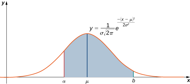
As mentioned above, the integral $\int e^{− x^{2}} d x$ arises often in probability theory. Specifically, it is used when studying data sets that are normally distributed, meaning the data values lie under a bell-shaped curve. For example, if a set of data values is normally distributed with mean $μ$ and standard deviation $σ,$ then the probability that a randomly chosen value lies between $x = a$ and $x = b$ is given by

\frac{1}{σ \sqrt{2 π}} \int_{a}^{b} e^{− {(x - μ)}^{2} / (2 σ^{2})} d x .

6.10

(See Figure 6.11.)

This graph is the normal distribution. It is a bell-shaped curve with the highest point above mu on the x-axis. Also, there is a shaded area under the curve above the x-axis. The shaded area is bounded by alpha on the left and b on the right. — Figure 6.11 If data values are normally distributed with mean $μ$ and standard deviation $σ,$ the probability that a randomly selected data value is between $a$ and $b$ is the area under the curve $y = \frac{1}{σ \sqrt{2 π}} e^{− {(x - μ)}^{2} / (2 σ^{2})}$ between $x = a$ and $x = b .$

To simplify this integral, we typically let $z = \frac{x - μ}{σ} .$ This quantity $z$ is known as the $z$ score of a data value. With this simplification, integral Equation 6.10 becomes

\frac{1}{\sqrt{2 π}} \int_{(a - μ) / σ}^{(b - μ) / σ} e^{− z^{2} / 2} d z .

6.11

In Example 6.23, we show how we can use this integral in calculating probabilities.

Using Maclaurin Series to Approximate a Probability

Suppose a set of standardized test scores are normally distributed with mean $μ = 100$ and standard deviation $σ = 50 .$ Use Equation 6.11 and the first six terms in the Maclaurin series for $e^{− x^{2} / 2}$ to approximate the probability that a randomly selected test score is between $x = 100$ and $x = 200 .$ Use the alternating series test to determine how accurate your approximation is.

Since $μ = 100, σ = 50,$ and we are trying to determine the area under the curve from $a = 100$ to $b = 200,$ integral Equation 6.11 becomes

\frac{1}{\sqrt{2 π}} \int_{0}^{2} e^{− z^{2} / 2} d z .

The Maclaurin series for $e^{− x^{2} / 2}$ is given by

\begin{matrix} e^{− x^{2} / 2} & = \sum_{n = 0}^{\infty} \frac{{(- \frac{x^{2}}{2})}^{n}}{n!} \\ = 1 - \frac{x^{2}}{2^{1} \cdot 1!} + \frac{x^{4}}{2^{2} \cdot 2!} - \frac{x^{6}}{2^{3} \cdot 3!} + ⋯ + {(−1)}^{n} \frac{x^{2 n}}{2^{n} \cdot n!} + ⋯ \\ = \sum_{n = 0}^{\infty} {(−1)}^{n} \frac{x^{2}^{n}}{2^{n} \cdot n!} . \end{matrix}

Therefore,

\begin{matrix} \frac{1}{\sqrt{2 π}} \int e^{− z^{2} / 2} d z & = & \frac{1}{\sqrt{2 π}} \int (1 - \frac{z^{2}}{2^{1} \cdot 1!} + \frac{z^{4}}{2^{2} \cdot 2!} - \frac{z^{6}}{2^{3} \cdot 3!} + ⋯ + {(−1)}^{n} \frac{z^{2 n}}{2^{n} \cdot n!} + ⋯) d z \\ = & \frac{1}{\sqrt{2 π}} (C + z - \frac{z^{3}}{3 \cdot 2^{1} \cdot 1!} + \frac{z^{5}}{5 \cdot 2^{2} \cdot 2!} - \frac{z^{7}}{7 \cdot 2^{3} \cdot 3!} + ⋯ + {(−1)}^{n} \frac{z^{2 n + 1}}{(2 n + 1) 2^{n} \cdot n!} + ⋯) \\ \frac{1}{\sqrt{2 π}} \int_{0}^{2} e^{− z^{2} / 2} d z & = & \frac{1}{\sqrt{2 π}} (2 - \frac{8}{6} + \frac{32}{40} - \frac{128}{336} + \frac{512}{3456} - \frac{2^{11}}{11 \cdot 2^{5} \cdot 5!} + ⋯) . \end{matrix}

Using the first five terms, we estimate that the probability is approximately $0.4922 .$ By the alternating series test, we see that this estimate is accurate to within

\frac{1}{\sqrt{2 π}} \frac{2^{13}}{13 \cdot 2^{6} \cdot 6!} \approx 0.00546 .

Analysis

If you are familiar with probability theory, you may know that the probability that a data value is within two standard deviations of the mean is approximately $95 % .$ Here we calculated the probability that a data value is between the mean and two standard deviations above the mean, so the estimate should be around $47.5 % .$ The estimate, combined with the bound on the accuracy, falls within this range.

Use the first five terms of the Maclaurin series for $e^{− x^{2} / 2}$ to estimate the probability that a randomly selected test score is between $100$ and $150 .$ Use the alternating series test to determine the accuracy of this estimate.

The estimate is approximately $0.3414 .$ This estimate is accurate to within $0.0000094 .$

Hint

Evaluate $\int_{0}^{1} e^{− z^{2} / 2} d z$ using the first five terms of the Maclaurin series for $e^{− z^{2} / 2} .$

Another application in which a nonelementary integral arises involves the period of a pendulum. The integral is

\int_{0}^{π / 2} \frac{d θ}{\sqrt{1 - k^{2} {sin}^{2} θ}} .

An integral of this form is known as an elliptic integral of the first kind. Elliptic integrals originally arose when trying to calculate the arc length of an ellipse. We now show how to use power series to approximate this integral.

Period of a Pendulum

The period of a pendulum is the time it takes for a pendulum to make one complete back-and-forth swing. For a pendulum with length $L$ that makes a maximum angle $θ_{max}$ with the vertical, its period $T$ is given by

T = 4 \sqrt{\frac{L}{g}} \int_{0}^{π / 2} \frac{d θ}{\sqrt{1 - k^{2} {sin}^{2} θ}}

where $g$ is the acceleration due to gravity and $k = sin (\frac{θ_{max}}{2})$ (see Figure 6.12). (We note that this formula for the period arises from a non-linearized model of a pendulum. In some cases, for simplification, a linearized model is used and $sin θ$ is approximated by $θ .)$ Use the binomial series

\frac{1}{\sqrt{1 + x}} = 1 + \sum_{n = 1}^{\infty} \frac{{(−1)}^{n}}{n!} \frac{1 \cdot 3 \cdot 5 ⋯ (2 n - 1)}{2^{n}} x^{n}

to estimate the period of this pendulum. Specifically, approximate the period of the pendulum if

you use only the first term in the binomial series, and
you use the first two terms in the binomial series.

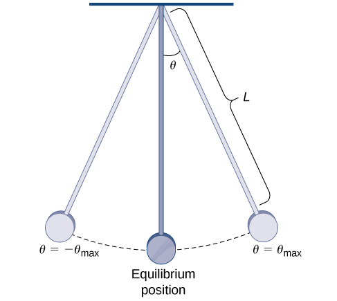
Figure 6.12 This pendulum has length $L$ and makes a maximum angle $θ_{max}$ with the vertical.

We use the binomial series, replacing $x$ with $− k^{2} {sin}^{2} θ .$ Then we can write the period as

T = 4 \sqrt{\frac{L}{g}} \int_{0}^{π / 2} (1 + \frac{1}{2} k^{2} {sin}^{2} θ + \frac{1 \cdot 3}{2! 2^{2}} k^{4} {sin}^{4} θ + ⋯) d θ .

Using just the first term in the integrand, the first-order estimate is

$T \approx 4 \sqrt{\frac{L}{g}} \int_{0}^{π / 2} d θ = 2 π \sqrt{\frac{L}{g}} .$

If $θ_{max}$ is small, then $k = sin (\frac{θ_{max}}{2})$ is small. We claim that when $k$ is small, this is a good estimate. To justify this claim, consider

$\int_{0}^{π / 2} (1 + \frac{1}{2} k^{2} {sin}^{2} θ + \frac{1 \cdot 3}{2! 2^{2}} k^{4} {sin}^{4} θ + ⋯) d θ .$

Since $| sin x | \leq 1,$ this integral is bounded by

$\int_{0}^{π / 2} (\frac{1}{2} k^{2} + \frac{1.3}{2! 2^{2}} k^{4} + ⋯) d θ < \frac{π}{2} (\frac{1}{2} k^{2} + \frac{1 \cdot 3}{2! 2^{2}} k^{4} + ⋯) .$

Furthermore, it can be shown that each coefficient on the right-hand side is less than $1$ and, therefore, that this expression is bounded by

$\frac{π k^{2}}{2} (1 + k^{2} + k^{4} + ⋯) = \frac{π k^{2}}{2} \cdot \frac{1}{1 - k^{2}},$

which is small for $k$ small.
For larger values of $θ_{max},$ we can approximate $T$ by using more terms in the integrand. By using the first two terms in the integral, we arrive at the estimate

$\begin{matrix} T & \approx 4 \sqrt{\frac{L}{g}} \int_{0}^{π / 2} (1 + \frac{1}{2} k^{2} {sin}^{2} θ) d θ \\ = 2 π \sqrt{\frac{L}{g}} (1 + \frac{k^{2}}{4}) . \end{matrix}$

The applications of Taylor series in this section are intended to highlight their importance. In general, Taylor series are useful because they allow us to represent known functions using polynomials, thus providing us a tool for approximating function values and estimating complicated integrals. In addition, they allow us to define new functions as power series, thus providing us with a powerful tool for solving differential equations.

Key Concepts

The binomial series is the Maclaurin series for $f (x) = {(1 + x)}^{r} .$ It converges for $| x | < 1 .$
Taylor series for functions can often be derived by algebraic operations with a known Taylor series or by differentiating or integrating a known Taylor series.
Power series can be used to solve differential equations.
Taylor series can be used to help approximate integrals that cannot be evaluated by other means.

In the following exercises, use appropriate substitutions to write down the Maclaurin series for the given binomial.

${(1 - x)}^{1 / 3}$

${(1 + x^{2})}^{−1 / 3}$

${(1 + x^{2})}^{−1 / 3} = \sum_{n = 0}^{\infty} (\begin{matrix} - \frac{1}{3} \\ n \end{matrix}) x^{2 n}$

${(1 - x)}^{1.01}$

${(1 - 2 x)}^{2 / 3}$

${(1 - 2 x)}^{2 / 3} = \sum_{n = 0}^{\infty} {(−1)}^{n} 2^{n} (\begin{matrix} \frac{2}{3} \\ n \end{matrix}) x^{n}$

In the following exercises, use the substitution ${(b + x)}^{r} = {(b + a)}^{r} {(1 + \frac{x - a}{b + a})}^{r}$ in the binomial expansion to find the Taylor series of each function with the given center.

$\sqrt{x + 2}$ at $a = 0$

$\sqrt{x^{2} + 2}$ at $a = 0$

$\sqrt{2 + x^{2}} = \sum_{n = 0}^{\infty} 2^{(1 / 2) - n} (\begin{matrix} \frac{1}{2} \\ n \end{matrix}) x^{2 n}; (| x^{2} | < 2)$

$\sqrt{x + 2}$ at $a = 1$

$\sqrt{2 x - x^{2}}$ at $a = 1$ (Hint: $2 x - x^{2} = 1 - {(x - 1)}^{2})$

$\sqrt{2 x - x^{2}} = \sqrt{1 - {(x - 1)}^{2}}$ so $\sqrt{2 x - x^{2}} = \sum_{n = 0}^{\infty} {(−1)}^{n} (\begin{matrix} \frac{1}{2} \\ n \end{matrix}) {(x - 1)}^{2 n}$

${(x - 8)}^{1 / 3}$ at $a = 9$

$\sqrt{x}$ at $a = 4$

$\sqrt{x} = 2 \sqrt{1 + \frac{x - 4}{4}}$ so $\sqrt{x} = \sum_{n = 0}^{\infty} 2^{1 - 2 n} (\begin{matrix} \frac{1}{2} \\ n \end{matrix}) {(x - 4)}^{n}$

$x^{1 / 3}$ at $a = 27$

$\sqrt{x}$ at $α = 9$

$\sqrt{x} = \sum_{n = 0}^{\infty} 3^{1 - 2 n} (\frac{1}{2} n) {(x - 9)}^{n}$

In the following exercises, use the binomial theorem to estimate each number, computing enough terms to obtain an estimate accurate to an error of at most $1 / 1000 .$

[T] ${(15)}^{1 / 4}$ using ${(16 - x)}^{1 / 4}$

[T] ${(1001)}^{1 / 3}$ using ${(1000 + x)}^{1 / 3}$

$10 {(1 + \frac{x}{1000})}^{1 / 3} = \sum_{n = 0}^{\infty} 10^{1 - 3 n} (\begin{matrix} \frac{1}{3} \\ n \end{matrix}) x^{n} .$ Using, for example, a fourth-degree estimate at $x = 1$ gives $\begin{matrix} {(1001)}^{1 / 3} & \approx 10 (1 + (\begin{matrix} \frac{1}{3} \\ 1 \end{matrix}) 10^{−3} + (\begin{matrix} \frac{1}{3} \\ 2 \end{matrix}) 10^{−6} + (\begin{matrix} \frac{1}{3} \\ 3 \end{matrix}) 10^{−9} + (\begin{matrix} \frac{1}{3} \\ 4 \end{matrix}) 10^{−12}) \\ = 10 (1 + \frac{1}{{3.10}^{3}} - \frac{1}{{9.10}^{6}} + \frac{5}{{81.10}^{9}} - \frac{10}{{243.10}^{12}}) = 10.00333222... \end{matrix}$ whereas ${(1001)}^{1 / 3} = 10.00332222839093 ....$ Two terms would suffice for three-digit accuracy.

In the following exercises, use the binomial approximation $\sqrt{1 - x} \approx 1 - \frac{x}{2} - \frac{x^{2}}{8} - \frac{x^{3}}{16} - \frac{5 x^{4}}{128} - \frac{7 x^{5}}{256}$ for $| x | < 1$ to approximate each number. Compare this value to the value given by a scientific calculator.

[T] $\frac{1}{\sqrt{2}}$ using $x = \frac{1}{2}$ in ${(1 - x)}^{1 / 2}$

[T] $\sqrt{5} = 5 \times \frac{1}{\sqrt{5}}$ using $x = \frac{4}{5}$ in ${(1 - x)}^{1 / 2}$

The approximation is $2.3152;$ the CAS value is $2.23 … .$

[T] $\sqrt{3} = \frac{3}{\sqrt{3}}$ using $x = \frac{2}{3}$ in ${(1 - x)}^{1 / 2}$

[T] $\sqrt{6}$ using $x = \frac{5}{6}$ in ${(1 - x)}^{1 / 2}$

The approximation is $2.583 …;$ the CAS value is $2.449 … .$

Integrate the binomial approximation of $\sqrt{1 - x}$ to find an approximation of $\int_{0}^{x} \sqrt{1 - t} d t .$

[T] Recall that the graph of $\sqrt{1 - x^{2}}$ is an upper semicircle of radius $1 .$ Integrate the binomial approximation of $\sqrt{1 - x^{2}}$ up to order $8$ from $x = −1$ to $x = 1$ to estimate $\frac{π}{2} .$

$\sqrt{1 - x^{2}} = 1 - \frac{x^{2}}{2} - \frac{x^{4}}{8} - \frac{x^{6}}{16} - \frac{5 x^{8}}{128} + ⋯ .$ Thus

$\int_{−1}^{1} \sqrt{1 - x^{2}} d x = x - \frac{x^{3}}{6} - \frac{x^{5}}{40} - \frac{x^{7}}{7 \cdot 16} - \frac{5 x^{9}}{9 \cdot 128} + ⋯ |_{−1}^{1} \approx 2 - \frac{1}{3} - \frac{1}{20} - \frac{1}{56} - \frac{10}{9 \cdot 128} + error = 1.590 ...$ whereas $\frac{π}{2} = 1.570 ...$

In the following exercises, use the expansion ${(1 + x)}^{1 / 3} = 1 + \frac{1}{3} x - \frac{1}{9} x^{2} + \frac{5}{81} x^{3} - \frac{10}{243} x^{4} + ⋯$ to write the first five terms (not necessarily a quartic polynomial) of each expression.

${(1 + 4 x)}^{1 / 3}; a = 0$

${(1 + 4 x)}^{4 / 3}; a = 0$

$\begin{array}{l} {(1 + 4 x)}^{4 / 3} = (1 + 4 x) {(1 + 4 x)}^{1 / 3} \\ = (1 + 4 x) (1 + \frac{4 x}{3} - \frac{16 x^{3}}{9} + \frac{320 x^{3}}{81} - \frac{2560 x^{4}}{243}) \\ = 1 + \frac{16}{3} x + \frac{32}{9} x^{2} - \frac{256}{81} x^{3} + \frac{1280}{243} x^{4} - \frac{10240}{243} x^{5} \end{array}$

${(3 + 2 x)}^{1 / 3}; a = −1$

${(x^{2} + 6 x + 10)}^{1 / 3}; a = −3$

${(1 + {(x + 3)}^{2})}^{1 / 3} = 1 + \frac{1}{3} {(x + 3)}^{2} - \frac{1}{9} {(x + 3)}^{4} + \frac{5}{81} {(x + 3)}^{6} - \frac{10}{243} {(x + 3)}^{8} + ⋯$

Use ${(1 + x)}^{1 / 3} = 1 + \frac{1}{3} x - \frac{1}{9} x^{2} + \frac{5}{81} x^{3} - \frac{10}{243} x^{4} + ⋯$ with $x = 1$ to approximate $2^{1 / 3} .$

Use the approximation ${(1 - x)}^{2 / 3} = 1 - \frac{2 x}{3} - \frac{x^{2}}{9} - \frac{4 x^{3}}{81} - \frac{7 x^{4}}{243} - \frac{14 x^{5}}{729} + ⋯$ for $| x | < 1$ to approximate $2^{1 / 3} = {2.2}^{−2 / 3} .$

Twice the approximation is $1.260 …$ whereas $2^{1 / 3} = 1.2599. ...$

Find the $25 th$ derivative of $f (x) = {(1 + x^{2})}^{13}$ at $x = 0 .$

Find the $99$ th derivative at $x = 0$ of $f (x) = {(1 + x^{4})}^{25} .$

$f^{(99)} (0) = 0$

In the following exercises, find the Maclaurin series of each function.

$f (x) = x e^{2 x}$

$f (x) = 2^{x}$

$\sum_{n = 0}^{\infty} \frac{{(ln (2) x)}^{n}}{n!}$

$f (x) = \frac{sin x}{x}$

$f (x) = \frac{sin (\sqrt{x})}{\sqrt{x}}, (x > 0),$

For $x > 0, sin (\sqrt{x}) = \sum_{n = 0}^{\infty} {(−1)}^{n} \frac{x^{(2 n + 1) / 2}}{\sqrt{x} (2 n + 1)!} = \sum_{n = 0}^{\infty} {(−1)}^{n} \frac{x^{n}}{(2 n + 1)!} .$

$f (x) = sin (x^{2})$

$f (x) = e^{x^{3}}$

$e^{x^{3}} = \sum_{n = 0}^{\infty} \frac{x^{3 n}}{n!}$

$f (x) = {cos}^{2} x$ using the identity ${cos}^{2} x = \frac{1}{2} + \frac{1}{2} cos (2 x)$

$f (x) = {sin}^{2} x$ using the identity ${sin}^{2} x = \frac{1}{2} - \frac{1}{2} cos (2 x)$

${sin}^{2} x = − \sum_{k = 1}^{\infty} \frac{{(−1)}^{k} 2^{2 k - 1} x^{2 k}}{(2 k)!}$

In the following exercises, find the Maclaurin series of $F (x) = \int_{0}^{x} f (t) d t$ by integrating the Maclaurin series of $f$ term by term. If $f$ is not strictly defined at zero, you may substitute the value of the Maclaurin series at zero.

$F (x) = \int_{0}^{x} e^{− t^{2}} d t; f (t) = e^{− t^{2}} = \sum_{n = 0}^{\infty} {(−1)}^{n} \frac{t^{2 n}}{n!}$

$F (x) = {tan}^{−1} x; f (t) = \frac{1}{1 + t^{2}} = \sum_{n = 0}^{\infty} {(−1)}^{n} t^{2 n}$

${tan}^{−1} x = \sum_{k = 0}^{\infty} \frac{{(−1)}^{k} x^{2 k + 1}}{2 k + 1}$

$F (x) = {tanh}^{−1} x; f (t) = \frac{1}{1 - t^{2}} = \sum_{n = 0}^{\infty} t^{2 n}$

$F (x) = {sin}^{−1} x; f (t) = \frac{1}{\sqrt{1 - t^{2}}} = \sum_{k = 0}^{\infty} (\begin{matrix} \frac{1}{2} \\ k \end{matrix}) \frac{t^{2 k}}{k!}$

${sin}^{−1} x = \sum_{n = 0}^{\infty} (\begin{matrix} \frac{1}{2} \\ n \end{matrix}) \frac{x^{2 n + 1}}{(2 n + 1) n!}$

$F (x) = \int_{0}^{x} \frac{sin t}{t} d t; f (t) = \frac{sin t}{t} = \sum_{n = 0}^{\infty} {(−1)}^{n} \frac{t^{2 n}}{(2 n + 1)!}$

$F (x) = \int_{0}^{x} cos (\sqrt{t}) d t; f (t) = \sum_{n = 0}^{\infty} {(−1)}^{n} \frac{x^{n}}{(2 n)!}$

$F (x) = \sum_{n = 0}^{\infty} {(−1)}^{n} \frac{x^{n + 1}}{(n + 1) (2 n)!}$

$F (x) = \int_{0}^{x} \frac{1 - cos t}{t^{2}} d t; f (t) = \frac{1 - cos t}{t^{2}} = \sum_{n = 0}^{\infty} {(−1)}^{n} \frac{t^{2 n}}{(2 n + 2)!}$

$F (x) = \int_{0}^{x} \frac{ln (1 + t)}{t} d t; f (t) = \sum_{n = 0}^{\infty} {(−1)}^{n} \frac{t^{n}}{n + 1}$

$F (x) = \sum_{n = 1}^{\infty} {(−1)}^{n + 1} \frac{x^{n}}{n^{2}}$

In the following exercises, compute at least the first three nonzero terms (not necessarily a quadratic polynomial) of the Maclaurin series of $f .$

$f (x) = sin (x + \frac{π}{4}) = sin x cos (\frac{π}{4}) + cos x sin (\frac{π}{4})$

$f (x) = tan x$

$x + \frac{x^{3}}{3} + \frac{2 x^{5}}{15} + ⋯$

$f (x) = ln (cos x)$

$f (x) = e^{x} cos x$

$1 + x - \frac{x^{3}}{3} - \frac{x^{4}}{6} + ⋯$

$f (x) = e^{sin x}$

$f (x) = {sec}^{2} x$

$1 + x^{2} + \frac{2 x^{4}}{3} + \frac{17 x^{6}}{45} + ⋯$

$f (x) = tanh x$

$f (x) = \frac{tan \sqrt{x}}{\sqrt{x}}$ (see expansion for $tan x)$

Using the expansion for $tan x$ gives $1 + \frac{x}{3} + \frac{2 x^{2}}{15} .$

In the following exercises, find the radius of convergence of the Maclaurin series of each function.

$ln (1 + x)$

$\frac{1}{1 + x^{2}}$

$\frac{1}{1 + x^{2}} = \sum_{n = 0}^{\infty} {(−1)}^{n} x^{2 n}$ so $R = 1$ by the ratio test.

${tan}^{−1} x$

$ln (1 + x^{2})$

$ln (1 + x^{2}) = \sum_{n = 1}^{\infty} \frac{{(−1)}^{n - 1}}{n} x^{2 n}$ so $R = 1$ by the ratio test.

Find the Maclaurin series of $sinh x = \frac{e^{x} - e^{− x}}{2} .$

Find the Maclaurin series of $cosh x = \frac{e^{x} + e^{− x}}{2} .$

Add series of $e^{x}$ and $e^{− x}$ term by term. Odd terms cancel and $cosh x = \sum_{n = 0}^{\infty} \frac{x^{2 n}}{(2 n)!} .$

Differentiate term by term the Maclaurin series of $sinh x$ and compare the result with the Maclaurin series of $cosh x .$

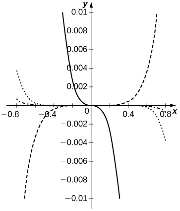
[T] Let $S_{n} (x) = \sum_{k = 0}^{n} {(−1)}^{k} \frac{x^{2 k + 1}}{(2 k + 1)!}$ and $C_{n} (x) = \sum_{n = 0}^{n} {(−1)}^{k} \frac{x^{2 k}}{(2 k)!}$ denote the respective Maclaurin polynomials of degree $2 n + 1$ of $sin x$ and degree $2 n$ of $cos x .$ Plot the errors $\frac{S_{n} (x)}{C_{n} (x)} - tan x$ for $n = 1, .., 5$ and compare them to $x + \frac{x^{3}}{3} + \frac{2 x^{5}}{15} + \frac{17 x^{7}}{315} - tan x$ on $(- \frac{π}{4}, \frac{π}{4}) .$

This graph has two curves. The first one is a decreasing function passing through the origin. The second is a broken line which is an increasing function passing through the origin. The two curves are very close around the origin.

The ratio $\frac{S_{n} (x)}{C_{n} (x)}$ approximates $tan x$ better than does $p_{7} (x) = x + \frac{x^{3}}{3} + \frac{2 x^{5}}{15} + \frac{17 x^{7}}{315}$ for $N \geq 3 .$ The dashed curves are $\frac{S_{n}}{C_{n}} - tan$ for $n = 1, 2 .$ The dotted curve corresponds to $n = 3,$ and the dash-dotted curve corresponds to $n = 4 .$ The solid curve is $p_{7} - tan x .$

Use the identity $2 sin x cos x = sin (2 x)$ to find the power series expansion of ${sin}^{2} x$ at $x = 0 .$ (Hint: Integrate the Maclaurin series of $sin (2 x)$ term by term.)

If $y = \sum_{n = 0}^{\infty} a_{n} x^{n},$ find the power series expansions of $x y^{'}$ and $x^{2} y^{″} .$

By the term-by-term differentiation theorem, $y^{'} = \sum_{n = 1}^{\infty} n a_{n} x^{n - 1}$ so $y^{'} = \sum_{n = 1}^{\infty} n a_{n} x^{n - 1} x y^{'} = \sum_{n = 1}^{\infty} n a_{n} x^{n},$ whereas $y^{'} = \sum_{n = 2}^{\infty} n (n - 1) a_{n} x^{n - 2}$ so $x y^{″} = \sum_{n = 2}^{\infty} n (n - 1) a_{n} x^{n} .$

[T] Suppose that $y = \sum_{k = 0}^{\infty} a_{k} x^{k}$ satisfies $y^{'} = −2 x y$ and $y (0) = 0 .$ Show that $a_{2 k + 1} = 0$ for all $k$ and that $a_{2 k + 2} = \frac{− a_{2 k}}{k + 1} .$ Plot the partial sum $S_{20}$ of $y$ on the interval $[−4, 4] .$

[T] Suppose that a set of standardized test scores is normally distributed with mean $μ = 100$ and standard deviation $σ = 10 .$ Set up an integral that represents the probability that a test score will be between $90$ and $110$ and use the integral of the degree $10$ Maclaurin polynomial of $\frac{1}{\sqrt{2 π}} e^{− x^{2} / 2}$ to estimate this probability.

The probability is $p = \frac{1}{\sqrt{2 π}} \int_{(a - μ) / σ}^{(b - μ) / σ} e^{− x^{2} / 2} d x$ where $a = 90$ and $b = 100,$ that is, $p = \frac{1}{\sqrt{2 π}} \int_{−1}^{1} e^{− x^{2} / 2} d x = \frac{1}{\sqrt{2 π}} \int_{−1}^{1} \sum_{n = 0}^{5} {(−1)}^{n} \frac{x^{2 n}}{2^{n} n!} d x = \frac{2}{\sqrt{2 π}} \sum_{n = 0}^{5} {(−1)}^{n} \frac{1}{(2 n + 1) 2^{n} n!} \approx 0.6827 .$

[T] Suppose that a set of standardized test scores is normally distributed with mean $μ = 100$ and standard deviation $σ = 10 .$ Set up an integral that represents the probability that a test score will be between $70$ and $130$ and use the integral of the degree $50$ Maclaurin polynomial of $\frac{1}{\sqrt{2 π}} e^{− x^{2} / 2}$ to estimate this probability.

[T] Suppose that $\sum_{n = 0}^{\infty} a_{n} x^{n}$ converges to a function $f (x)$ such that $f (0) = 1, f^{'} (0) = 0,$ and $f^{″} (x) = − f (x) .$ Find a formula for $a_{n}$ and plot the partial sum $S_{N}$ for $N = 20$ on $[−5, 5] .$

This graph is a wave curve symmetrical about the origin. It has a peak at y = 1 above the origin. It has lowest points at -3 and 3.

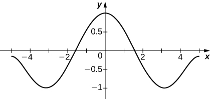
As in the previous problem one obtains $a_{n} = 0$ if $n$ is odd and $a_{n} = − (n + 2) (n + 1) a_{n + 2}$ if $n$ is even, so $a_{0} = 1$ leads to $a_{2 n} = \frac{{(−1)}^{n}}{(2 n)!} .$

[T] Suppose that $\sum_{n = 0}^{\infty} a_{n} x^{n}$ converges to a function $f (x)$ such that $f (0) = 0, f^{'} (0) = 1,$ and $f^{″} (x) = − f (x) .$ Find a formula for $a_{n}$ and plot the partial sum $S_{N}$ for $N = 10$ on $[−5, 5] .$

Suppose that $\sum_{n = 0}^{\infty} a_{n} x^{n}$ converges to a function $y$ such that $y^{″} - y^{'} + y = 0$ where $y (0) = 1$ and $y' (0) = 0 .$ Find a formula that relates $a_{n + 2}, a_{n + 1},$ and $a_{n}$ and compute $a_{0}, ..., a_{5} .$

$y^{″} = \sum_{n = 0}^{\infty} (n + 2) (n + 1) a_{n + 2} x^{n}$ and $y^{'} = \sum_{n = 0}^{\infty} (n + 1) a_{n + 1} x^{n}$ so $y^{″} - y^{'} + y = 0$ implies that $(n + 2) (n + 1) a_{n + 2} - (n + 1) a_{n + 1} + a_{n} = 0$ or $a_{n} = \frac{a_{n - 1}}{n} - \frac{a_{n - 2}}{n (n - 1)}$ for all $n \cdot y (0) = a_{0} = 1$ and $y^{'} (0) = a_{1} = 0,$ so $a_{2} = \frac{1}{2}, a_{3} = \frac{1}{6}, a_{4} = 0,$ and $a_{5} = - \frac{1}{120} .$

Suppose that $\sum_{n = 0}^{\infty} a_{n} x^{n}$ converges to a function $y$ such that $y^{″} - y^{'} + y = 0$ where $y (0) = 0$ and $y^{'} (0) = 1 .$ Find a formula that relates $a_{n + 2}, a_{n + 1},$ and $a_{n}$ and compute $a_{1}, ..., a_{5} .$

The error in approximating the integral $\int_{a}^{b} f (t) d t$ by that of a Taylor approximation $\int_{a}^{b} P_{n} (t) d t$ is at most $\int_{a}^{b} R_{n} (t) d t .$ In the following exercises, the Taylor remainder estimate $R_{n} \leq \frac{M}{(n + 1)!} {| x - a |}^{n + 1}$ guarantees that the integral of the Taylor polynomial of the given order approximates the integral of $f$ with an error less than $\frac{1}{10} .$

Evaluate the integral of the appropriate Taylor polynomial and verify that it approximates the CAS value with an error less than $\frac{1}{100} .$
Compare the accuracy of the polynomial integral estimate with the remainder estimate.

[T] $\int_{0}^{π} \frac{sin t}{t} d t; P_{s} = 1 - \frac{x^{2}}{3!} + \frac{x^{4}}{5!} - \frac{x^{6}}{7!} + \frac{x^{8}}{9!}$ (You may assume that the absolute value of the ninth derivative of $\frac{sin t}{t}$ is bounded by $0.1 .)$

a. (Proof) b. We have $R_{s} \leq \frac{0.1}{(9)!} π^{9} \approx 0.0082 < 0.01 .$ We have $\int_{0}^{π} (1 - \frac{x^{2}}{3!} + \frac{x^{4}}{5!} - \frac{x^{6}}{7!} + \frac{x^{8}}{9!}) d x = π - \frac{π^{3}}{3 \cdot 3!} + \frac{π^{5}}{5 \cdot 5!} - \frac{π^{7}}{7 \cdot 7!} + \frac{π^{9}}{9 \cdot 9!} = 1.852...,$ whereas $\int_{0}^{π} \frac{sin t}{t} d t = 1.85194...,$ so the actual error is approximately $0.00006 .$

[T] $\int_{0}^{2} e^{− x^{2}} d x; p_{11} = 1 - x^{2} + \frac{x^{4}}{2} - \frac{x^{6}}{3!} + ⋯ - \frac{x^{22}}{11!}$ (You may assume that the absolute value of the $23 rd$ derivative of $e^{− x^{2}}$ is less than $2 \times 10^{14} .)$

The following exercises deal with Fresnel integrals.

The Fresnel integrals are defined by $C (x) = \int_{0}^{x} cos (t^{2}) d t$ and $S (x) = \int_{0}^{x} sin (t^{2}) d t .$ Compute the power series of $C (x)$ and $S (x)$ and plot the sums $C_{N} (x)$ and $S_{N} (x)$ of the first $N = 50$ nonzero terms on $[0, 2 π] .$

This graph has two curves. The first one is a solid curve labeled Csub50(x). It begins at the origin and is a wave that gradually decreases in amplitude. The highest it reaches is y = 1. The second curve is labeled Ssub50(x). It is a wave that gradually decreases in amplitude. The highest it reaches is 0.9. It is very close to the pattern of the first curve with a slight shift to the right.

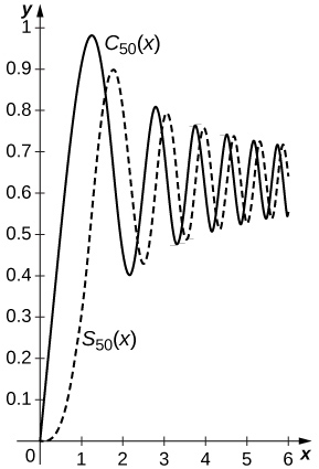
Since $cos (t^{2}) = \sum_{n = 0}^{\infty} {(−1)}^{n} \frac{t^{4 n}}{(2 n)!}$ and $sin (t^{2}) = \sum_{n = 0}^{\infty} {(−1)}^{n} \frac{t^{4 n + 2}}{(2 n + 1)!},$ one has $S (x) = \sum_{n = 0}^{\infty} {(−1)}^{n} \frac{x^{4 n + 3}}{(4 n + 3) (2 n + 1)!}$ and $C (x) = \sum_{n = 0}^{\infty} {(−1)}^{n} \frac{x^{4 n + 1}}{(4 n + 1) (2 n)!} .$ The sums of the first $50$ nonzero terms are plotted below with $C_{50} (x)$ the solid curve and $S_{50} (x)$ the dashed curve.

[T] The Fresnel integrals are used in design applications for roadways and railways and other applications because of the curvature properties of the curve with coordinates $(C (t), S (t)) .$ Plot the curve $(C_{50}, S_{50})$ for $0 \leq t \leq 2 π,$ the coordinates of which were computed in the previous exercise.

Estimate $\int_{0}^{1 / 4} \sqrt{x - x^{2}} d x$ by approximating $\sqrt{1 - x}$ using the binomial approximation $1 - \frac{x}{2} - \frac{x^{2}}{8} - \frac{x^{3}}{16} - \frac{5 x^{4}}{2128} - \frac{7 x^{5}}{256} .$

$\int_{0}^{1 / 4} \sqrt{x} (1 - \frac{x}{2} - \frac{x^{2}}{8} - \frac{x^{3}}{16} - \frac{5 x^{4}}{128} - \frac{7 x^{5}}{256}) d x$

$= \frac{2}{3} 2^{−3} - \frac{1}{2} \frac{2}{5} 2^{−5} - \frac{1}{8} \frac{2}{7} 2^{−7} - \frac{1}{16} \frac{2}{9} 2^{−9} - \frac{5}{128} \frac{2}{11} 2^{−11} - \frac{7}{256} \frac{2}{13} 2^{−13} = 0.0767732 ...$

whereas $\int_{0}^{1 / 4} \sqrt{x - x^{2}} d x = 0.076773 .$

[T] Use Newton’s approximation of the binomial $\sqrt{1 - x^{2}}$ to approximate $π$ as follows. The circle centered at $(\frac{1}{2}, 0)$ with radius $\frac{1}{2}$ has upper semicircle $y = \sqrt{x} \sqrt{1 - x} .$ The sector of this circle bounded by the $x$ -axis between $x = 0$ and $x = \frac{1}{2}$ and by the line joining $(\frac{1}{4}, \frac{\sqrt{3}}{4})$ corresponds to $\frac{1}{6}$ of the circle and has area $\frac{π}{24} .$ This sector is the union of a right triangle with height $\frac{\sqrt{3}}{4}$ and base $\frac{1}{4}$ and the region below the graph between $x = 0$ and $x = \frac{1}{4} .$ To find the area of this region you can write $y = \sqrt{x} \sqrt{1 - x} = \sqrt{x} \times (binomial expansion of \sqrt{1 - x})$ and integrate term by term. Use this approach with the binomial approximation from the previous exercise to estimate $π .$

Use the approximation $T \approx 2 π \sqrt{\frac{L}{g}} (1 + \frac{k^{2}}{4})$ to approximate the period of a pendulum having length $10$ meters and maximum angle $θ_{max} = \frac{π}{6}$ where $k = sin (\frac{θ_{max}}{2}) .$ Compare this with the small angle estimate $T \approx 2 π \sqrt{\frac{L}{g}} .$

$T \approx 2 π \sqrt{\frac{10}{9.8}} (1 + \frac{{sin}^{2} (θ / 12)}{4}) \approx 6.453$ seconds. The small angle estimate is $T \approx 2 π \sqrt{\frac{10}{9.8} \approx 6.347} .$ The relative error is around $2$ percent.

Suppose that a pendulum is to have a period of $2$ seconds and a maximum angle of $θ_{max} = \frac{π}{6} .$ Use $T \approx 2 π \sqrt{\frac{L}{g}} (1 + \frac{k^{2}}{4})$ to approximate the desired length of the pendulum. What length is predicted by the small angle estimate $T \approx 2 π \sqrt{\frac{L}{g}} ?$

Evaluate $\int_{0}^{π / 2} {sin}^{4} θ d θ$ in the approximation $T = 4 \sqrt{\frac{L}{g}} \int_{0}^{π / 2} (1 + \frac{1}{2} k^{2} {sin}^{2} θ + \frac{3}{8} k^{4} {sin}^{4} θ + ⋯) d θ$ to obtain an improved estimate for $T .$

$\int_{0}^{π / 2} {sin}^{4} θ d θ = \frac{3 π}{16} .$ Hence $T \approx 2 π \sqrt{\frac{L}{g}} (1 + \frac{k^{2}}{4} + \frac{9}{256} k^{4}) .$

[T] An equivalent formula for the period of a pendulum with amplitude $θ_{max}$ is $T (θ_{max}) = 2 \sqrt{2} \sqrt{\frac{L}{g}} \int_{0}^{θ_{max}} \frac{d θ}{\sqrt{cos θ} - cos (θ_{max})}$ where $L$ is the pendulum length and $g$ is the gravitational acceleration constant. When $θ_{max} = \frac{π}{3}$ we get $\frac{1}{\sqrt{cos t - 1 / 2}} \approx \sqrt{2} (1 + \frac{t^{2}}{2} + \frac{t^{4}}{3} + \frac{181 t^{6}}{720}) .$ Integrate this approximation to estimate $T (\frac{π}{3})$ in terms of $L$ and $g .$ Assuming $g = 9.806$ meters per second squared, find an approximate length $L$ such that $T (\frac{π}{3}) = 2$ seconds.

Chapter Review Exercises

True or False? In the following exercises, justify your answer with a proof or a counterexample.

If the radius of convergence for a power series $\sum_{n = 0}^{\infty} a_{n} x^{n}$ is $5,$ then the radius of convergence for the series $\sum_{n = 1}^{\infty} n a_{n} x^{n - 1}$ is also $5 .$

True

Power series can be used to show that the derivative of $e^{x} is e^{x} .$ (Hint: Recall that $e^{x} = \sum_{n = 0}^{\infty} \frac{1}{n!} x^{n} .)$

For small values of $x, sin x \approx x .$

True

The radius of convergence for the Maclaurin series of $f (x) = 3^{x}$ is $3 .$

In the following exercises, find the radius of convergence and the interval of convergence for the given series.

$\sum_{n = 0}^{\infty} n^{2} {(x - 1)}^{n}$

ROC: $1;$ IOC: $(0, 2)$

$\sum_{n = 0}^{\infty} \frac{x^{n}}{n^{n}}$

$\sum_{n = 0}^{\infty} \frac{3 n x^{n}}{12^{n}}$

ROC: $12;$ IOC: $(−12, 12)$

$\sum_{n = 0}^{\infty} \frac{2^{n}}{e^{n}} {(x - e)}^{n}$

In the following exercises, find the power series representation for the given function. Determine the radius of convergence and the interval of convergence for that series.

$f (x) = \frac{x^{2}}{x + 3}$

$\sum_{n = 0}^{\infty} \frac{{(−1)}^{n}}{3^{n + 1}} x^{n + 2};$ ROC: $3;$ IOC: $(−3, 3)$

$f (x) = \frac{8 x + 2}{2 x^{2} - 3 x + 1}$

In the following exercises, find the power series for the given function using term-by-term differentiation or integration.

$f (x) = {tan}^{−1} (2 x)$

integration: $\sum_{n = 0}^{\infty} \frac{{(−1)}^{n}}{2 n + 1} {(2 x)}^{2 n + 1}$

$f (x) = \frac{x}{{(2 + x^{2})}^{2}}$

In the following exercises, evaluate the Taylor series expansion of degree four for the given function at the specified point. What is the error in the approximation?

$f (x) = x^{3} - 2 x^{2} + 4, a = −3$

$p_{4} (x) = {(x + 3)}^{3} - 11 {(x + 3)}^{2} + 39 (x + 3) - 41;$ exact

$f (x) = e^{1 / (4 x)}, a = 4$

In the following exercises, find the Maclaurin series for the given function.

$f (x) = cos (3 x)$

$\sum_{n = 0}^{\infty} \frac{{(−1)}^{n} {(3 x)}^{2 n}}{2 n!}$

$f (x) = ln (x + 1)$

In the following exercises, find the Taylor series at the given value.

$f (x) = sin x, a = \frac{π}{2}$

$\sum_{n = 0}^{\infty} \frac{{(−1)}^{n}}{(2 n)!} {(x - \frac{π}{2})}^{2 n}$

$f (x) = \frac{3}{x}, a = 1$

In the following exercises, find the Maclaurin series for the given function.

$f (x) = e^{− x^{2}} - 1$

$\sum_{n = 1}^{\infty} \frac{{(−1)}^{n}}{n!} x^{2 n}$

$f (x) = cos x - x sin x$

In the following exercises, find the Maclaurin series for $F (x) = \int_{0}^{x} f (t) d t$ by integrating the Maclaurin series of $f (x)$ term by term.

$f (x) = \frac{sin x}{x}$

$F (x) = \sum_{n = 0}^{\infty} \frac{{(−1)}^{n}}{(2 n + 1) (2 n + 1)!} x^{2 n + 1}$

$f (x) = 1 - e^{x}$

Use power series to prove Euler’s formula: $e^{i x} = cos x + i sin x$

Answers may vary.

The following exercises consider problems of annuity payments.

For annuities with a present value of $$ 1$ million, calculate the annual payouts given over $25$ years assuming interest rates of $1 %, 5 %, and 10 % .$

A lottery winner has an annuity that has a present value of $$ 10$ million. What interest rate would they need to live on perpetual annual payments of $$ 250,000 ?$

$2.5 %$

Calculate the necessary present value of an annuity in order to support annual payouts of $$ 15,000$ given over $25$ years assuming interest rates of $1 %, 5 %, and 10 % .$

Glossary

binomial series: the Maclaurin series for $f (x) = {(1 + x)}^{r};$ it is given by
${(1 + x)}^{r} = \sum_{n = 0}^{\infty} (\begin{matrix} r \\ n \end{matrix}) x^{n} = 1 + r x + \frac{r (r - 1)}{2!} x^{2} + ⋯ + \frac{r (r - 1) ⋯ (r - n + 1)}{n!} x^{n} + ⋯$ for $| x | < 1$
nonelementary integral: an integral for which the antiderivative of the integrand cannot be expressed as an elementary function