- Evaluate an integral over an infinite interval.
- Evaluate an integral over a closed interval with an infinite discontinuity within the interval.
- Use the comparison theorem to determine whether a definite integral is convergent.
Is the area between the graph of and the x-axis over the interval finite or infinite? If this same region is revolved about the x-axis, is the volume finite or infinite? Surprisingly, the area of the region described is infinite, but the volume of the solid obtained by revolving this region about the x-axis is finite.
In this section, we define integrals over an infinite interval as well as integrals of functions containing a discontinuity on the interval. Integrals of these types are called improper integrals. We examine several techniques for evaluating improper integrals, all of which involve taking limits.
Integrating over an Infinite Interval
How should we go about defining an integral of the type We can integrate for any value of so it is reasonable to look at the behavior of this integral as we substitute larger values of Figure 3.17 shows that may be interpreted as area for various values of In other words, we may define an improper integral as a limit, taken as one of the limits of integration increases or decreases without bound.

- Let be continuous over an interval of the form Then
3.16
provided this limit exists. - Let be continuous over an interval of the form Then
3.17
provided this limit exists.
In each case, if the limit exists, then the improper integral is said to converge. If the limit does not exist, then the improper integral is said to diverge. - Let be continuous over Then
3.18
provided that and both converge. If either one or both of these two integrals diverge, then diverges. (It can be shown that, in fact, for any value of
In our first example, we return to the question we posed at the start of this section: Is the area between the graph of and the -axis over the interval finite or infinite?
Determine whether the area between the graph of and the x-axis over the interval is finite or infinite.
We first do a quick sketch of the region in question, as shown in the following graph.
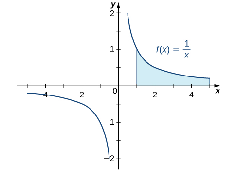
We can see that the area of this region is given by Then we have
Since the improper integral diverges to the area of the region is infinite.
Find the volume of the solid obtained by revolving the region bounded by the graph of and the x-axis over the interval about the -axis.
The solid is shown in Figure 3.19. Using the disk method, we see that the volume V is
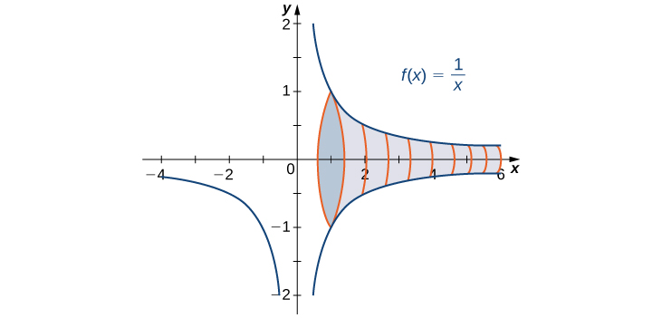
Then we have
The improper integral converges to Therefore, the volume of the solid of revolution is
In conclusion, although the area of the region between the x-axis and the graph of over the interval is infinite, the volume of the solid generated by revolving this region about the x-axis is finite. The solid generated is known as Gabriel’s Horn.
Visit this website to read more about Gabriel’s Horn.

In the chapter opener, we stated the following problem: Suppose that at a busy intersection, traffic accidents occur at an average rate of one every three months. After residents complained, changes were made to the traffic lights at the intersection. It has now been ten months since the changes were made and there have been no accidents. Were the changes effective or is the 10-month interval without an accident a result of chance?
Revise to: Let represent the amount of time it takes for the next accident to occur. We want to know how likely it is that . Define the rate parameter to be the average number of accidents per month. According to probability theory, for ,
In this example, since one accident happens every three months, on average, . The desired probability is:
The value represents the probability of no accidents in 8 months under the initial conditions. Since this value is very, very small, it is reasonable to conclude the changes were effective.
Evaluate State whether the improper integral converges or diverges.
Begin by rewriting as a limit using Equation 3.17 from the definition. Thus,
The improper integral converges to
Evaluate State whether the improper integral converges or diverges.
Start by splitting up the integral:
If either or diverges, then diverges. Compute each integral separately. For the first integral,
The first improper integral converges. For the second integral,
Thus, diverges. Since this integral diverges, diverges as well.
Evaluate State whether the improper integral converges or diverges.
converges
Integrating a Discontinuous Integrand
Now let’s examine integrals of functions containing an infinite discontinuity in the interval over which the integration occurs. Consider an integral of the form where is continuous over and discontinuous at Since the function is continuous over for all values of satisfying the integral is defined for all such values of Thus, it makes sense to consider the values of as approaches for That is, we define provided this limit exists. Figure 3.21 illustrates as areas of regions for values of approaching
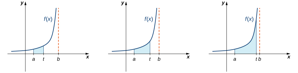
We use a similar approach to define where is continuous over and discontinuous at We now proceed with a formal definition.
- Let be continuous over Then,
3.19 - Let be continuous over Then,
3.20
In each case, if the limit exists, then the improper integral is said to converge. If the limit does not exist, then the improper integral is said to diverge. - If is continuous over except at a point in then
3.21
provided both and converge. If either of these integrals diverges, then diverges.
The following examples demonstrate the application of this definition.
Evaluate if possible. State whether the integral converges or diverges.
The function is continuous over and discontinuous at 4. Using Equation 3.19 from the definition, rewrite as a limit:
The improper integral converges.
Evaluate State whether the integral converges or diverges.
Since is continuous over and is discontinuous at zero, we can rewrite the integral in limit form using Equation 3.20:
The improper integral converges.
Evaluate State whether the improper integral converges or diverges.
Since is discontinuous at zero, using Equation 3.21, we can write
If either of the two integrals diverges, then the original integral diverges. Begin with
Therefore, diverges. Since diverges, diverges.
Evaluate State whether the integral converges or diverges.
diverges
Write in limit form using Equation 3.20.
A Comparison Theorem
It is not always easy or even possible to evaluate an improper integral directly; however, by comparing it with another carefully chosen integral, it may be possible to determine its convergence or divergence. To see this, consider two continuous functions and satisfying for (Figure 3.22). In this case, we may view integrals of these functions over intervals of the form as areas, so we have the relationship
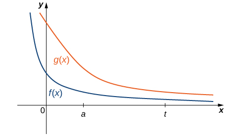
Thus, if
then
as well. That is, if the area of the region between the graph of and the x-axis over is infinite, then the area of the region between the graph of and the x-axis over is infinite too.
On the other hand, if
for some real number then
must converge to some value less than or equal to since increases as increases and for all
If the area of the region between the graph of and the x-axis over is finite, then the area of the region between the graph of and the x-axis over is also finite.
These conclusions are summarized in the following theorem.
Let and be continuous over Assume that for
- If then
- If where is a real number, then for some real number
Use a comparison to show that converges.
We can see that
so if converges, then so does To evaluate first rewrite it as a limit:
Since converges, so does
Use the comparison theorem to show that diverges for all
For over In Example 3.47, we showed that Therefore, diverges for all
Use a comparison to show that diverges.
Since diverges.
on
In the last few chapters, we have looked at several ways to use integration for solving real-world problems. For this next project, we are going to explore a more advanced application of integration: integral transforms. Specifically, we describe the Laplace transform and some of its properties. The Laplace transform is used in engineering and physics to simplify the computations needed to solve some problems. It takes functions expressed in terms of time and transforms them to functions expressed in terms of frequency. It turns out that, in many cases, the computations needed to solve problems in the frequency domain are much simpler than those required in the time domain.
The Laplace transform is defined in terms of an integral as
Note that the input to a Laplace transform is a function of time, and the output is a function of frequency, Although many real-world examples require the use of complex numbers (involving the imaginary number in this project we limit ourselves to functions of real numbers.
Let’s start with a simple example. Here we calculate the Laplace transform of . We have
This is an improper integral, so we express it in terms of a limit, which gives
Now we use integration by parts to evaluate the integral. Note that we are integrating with respect to t, so we treat the variable s as a constant. We have
Then we obtain
- Calculate the Laplace transform of
- Calculate the Laplace transform of
- Calculate the Laplace transform of (Note, you will have to integrate by parts twice.)
Laplace transforms are often used to solve differential equations. Differential equations are not covered in detail until later in this book; but, for now, let’s look at the relationship between the Laplace transform of a function and the Laplace transform of its derivative.
Let’s start with the definition of the Laplace transform. We have
- Use integration by parts to evaluate (Let and
After integrating by parts and evaluating the limit, you should see that
Then,
Thus, differentiation in the time domain simplifies to multiplication by s in the frequency domain.
The final thing we look at in this project is how the Laplace transforms of and its antiderivative are related. Let Then,
- Use integration by parts to evaluate (Let and Note, by the way, that we have defined
As you might expect, you should see that
Integration in the time domain simplifies to division by s in the frequency domain.
Key Concepts
- Integrals of functions over infinite intervals are defined in terms of limits.
- Integrals of functions over an interval for which the function has a discontinuity at an endpoint may be defined in terms of limits.
- The convergence or divergence of an improper integral may be determined by comparing it with the value of an improper integral for which the convergence or divergence is known.
Key Equations
| Improper integrals |
.
Evaluate the following integrals. If the integral is not convergent, answer “divergent.”
divergent
Without integrating, determine whether the integral converges or diverges by comparing the function with
Converges
Without integrating, determine whether the integral converges or diverges.
Determine whether the improper integrals converge or diverge. If possible, determine the value of the integrals that converge.
Converges to 1/2.
−4
diverges
diverges
1.5
diverges
diverges
diverges
Determine the convergence of each of the following integrals by comparison with the given integral. If the integral converges, find the number to which it converges.
compare with
compare with
Both integrals diverge.
Evaluate the integrals. If the integral diverges, answer “diverges.”
diverges
diverges
0.0
0.0
Evaluate the improper integrals. Each of these integrals has an infinite discontinuity either at an endpoint or at an interior point of the interval.
6.0
Evaluate (Be careful!) (Express your answer using three decimal places.)
Evaluate (Express the answer in exact form.)
Evaluate
Find the area of the region in the first quadrant between the curve and the x-axis.
Find the area of the region bounded by the curve the x-axis, and on the left by
7.0
Find the area under the curve bounded on the left by
Find the area under in the first quadrant.
Find the volume of the solid generated by revolving about the x-axis the region under the curve from to
Find the volume of the solid generated by revolving about the y-axis the region under the curve in the first quadrant.
Find the volume of the solid generated by revolving about the x-axis the area under the curve in the first quadrant.
The Laplace transform of a continuous function over the interval is defined by (see the Student Project). This definition is used to solve some important initial-value problems in differential equations, as discussed later. The domain of F is the set of all real numbers s such that the improper integral converges. Find the Laplace transform F of each of the following functions and give the domain of F.
Use the formula for arc length to show that the circumference of the circle is
Answers will vary.
A non-negative function is a probability density function if it satisfies the following definition: The probability that a random variable x lies between a and b is given by
Show that is a probability density function.
Find the probability that x is between 0 and 0.3. (Use the function defined in the preceding problem.) Use four-place decimal accuracy.
0.8775
Chapter Review Exercises
For the following exercises, determine whether the statement is true or false. Justify your answer with a proof or a counterexample.
cannot be integrated by parts.
cannot be integrated using partial fractions.
False
In numerical integration, increasing the number of points decreases the error.
Integration by parts can always yield the integral.
False
For the following exercises, evaluate the integral using the specified method.
using integration by parts
using trigonometric substitution
using integration by parts
using partial fractions
using trigonometric substitution
using a table of integrals or a CAS
For the following exercises, integrate using whatever method you choose.
For the following exercises, approximate the integrals using the midpoint rule, trapezoidal rule, and Simpson’s rule using four subintervals, rounding to three decimals.
[T]
[T]
[T]
For the following exercises, evaluate the integrals, if possible.
for what values of does this integral converge or diverge?
approximately 0.2194
For the following exercises, consider the gamma function given by
Show that
Extend to show that assuming is a positive integer.
The fastest car in the world, the Bugati Veyron, can reach a top speed of 408 km/h. The graph represents its velocity.
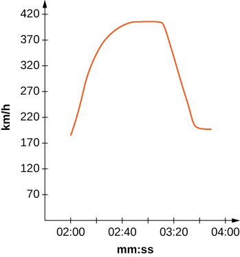
[T] Use the graph to estimate the velocity every 20 sec and fit to a graph of the form (Hint: Consider the time units.)
[T] Using your function from the previous problem, find exactly how far the Bugati Veyron traveled in the 1 min 40 sec included in the graph.
Answers may vary. Ex: km
Glossary
- improper integral
- an integral over an infinite interval or an integral of a function containing an infinite discontinuity on the interval; an improper integral is defined in terms of a limit. The improper integral converges if this limit is a finite real number; otherwise, the improper integral diverges