3.6 Numerical Integration

Approximate the value of a definite integral by using the midpoint and trapezoidal rules.
Determine the absolute and relative error in using a numerical integration technique.
Estimate the absolute and relative error using an error-bound formula.
Recognize when the midpoint and trapezoidal rules over- or underestimate the true value of an integral.
Use Simpson’s rule to approximate the value of a definite integral to a given accuracy.

The antiderivatives of many functions either cannot be expressed or cannot be expressed easily in closed form (that is, in terms of known functions). Consequently, rather than evaluate definite integrals of these functions directly, we resort to various techniques of numerical integration to approximate their values. In this section we explore several of these techniques. In addition, we examine the process of estimating the error in using these techniques.

The Midpoint Rule

Earlier in this text we defined the definite integral of a function over an interval as the limit of Riemann sums. In general, any Riemann sum of a function $f (x)$ over an interval $[a, b]$ may be viewed as an estimate of $\int_{a}^{b} f (x) d x .$ Recall that a Riemann sum of a function $f (x)$ over an interval $[a, b]$ is obtained by selecting a partition

P = {x_{0}, x_{1}, x_{2},…, x_{n}}, where a = x_{0} < x_{1} < x_{2} < \dots < x_{n} = b

and a set

S = {x_{1}^{*}, x_{2}^{*},…, x_{n}^{*}}, where x_{i - 1} \leq x_{i}^{*} \leq x_{i} for all i .

The Riemann sum corresponding to the partition $P$ and the set $S$ is given by $\sum_{i = 1}^{n} f (x_{i}^{*}) Δ x_{i},$ where $Δ x_{i} = x_{i} - x_{i - 1},$ the length of the ith subinterval.

The midpoint rule for estimating a definite integral uses a Riemann sum with subintervals of equal width and the midpoints, $m_{i},$ of each subinterval in place of $x_{i}^{*} .$ Formally, we state a theorem regarding the convergence of the midpoint rule as follows.

The Midpoint Rule

Assume that $f (x)$ is continuous on $[a, b] .$ Let n be a positive integer and $Δ x = \frac{b - a}{n} .$ If $[a, b]$ is divided into $n$ subintervals, each of length $Δ x,$ and $m_{i}$ is the midpoint of the ith subinterval, set

M_{n} = \sum_{i = 1}^{n} f (m_{i}) Δ x .

3.10

Then $lim_{n \to \infty} M_{n} = \int_{a}^{b} f (x) d x .$

As we can see in Figure 3.13, if $f (x) \geq 0$ over $[a, b],$ then $\sum_{i = 1}^{n} f (m_{i}) Δ x$ corresponds to the sum of the areas of rectangles approximating the area between the graph of $f (x)$ and the x-axis over $[a, b] .$ The graph shows the rectangles corresponding to $M_{4}$ for a nonnegative function over a closed interval $[a, b] .$

This figure is a graph of a non-negative function in the first quadrant. The function increases and decreases. The quadrant is divided into a grid. Beginning on the x-axis at the point labeled a = x sub 0, there are rectangles shaded whose heights are approximately the height of the curve. The x-axis is scaled by increments of msub1, x sub 1, m sub 2, x sub 2, m sub 3, x sub 3, m sub 4 and b = x sub 4. — Figure 3.13 The midpoint rule approximates the area between the graph of $f (x)$ and the x-axis by summing the areas of rectangles with midpoints that are points on $f (x) .$

Using the Midpoint Rule with

M_{4}

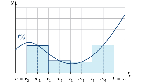
Use the midpoint rule to estimate $\int_{0}^{1} x^{2} d x$ using four subintervals. Compare the result with the actual value of this integral.

Each subinterval has length $Δ x = \frac{1 - 0}{4} = \frac{1}{4} .$ Therefore, the subintervals consist of

[0, \frac{1}{4}], [\frac{1}{4}, \frac{1}{2}], [\frac{1}{2}, \frac{3}{4}], and [\frac{3}{4}, 1] .

The midpoints of these subintervals are ${\frac{1}{8}, \frac{3}{8}, \frac{5}{8}, \frac{7}{8}} .$ Thus,

M_{4} = \frac{1}{4} f (\frac{1}{8}) + \frac{1}{4} f (\frac{3}{8}) + \frac{1}{4} f (\frac{5}{8}) + \frac{1}{4} f (\frac{7}{8}) = \frac{1}{4} \cdot \frac{1}{64} + \frac{1}{4} \cdot \frac{9}{64} + \frac{1}{4} \cdot \frac{25}{64} + \frac{1}{4} \cdot \frac{49}{64} = \frac{21}{64} .

Since

\int_{0}^{1} x^{2} d x = \frac{1}{3} and | \frac{1}{3} - \frac{21}{64} | = \frac{1}{192} \approx 0.0052,

we see that the midpoint rule produces an estimate that is somewhat close to the actual value of the definite integral.

Using the Midpoint Rule with

M_{6}

Use $M_{6}$ to estimate the length of the curve $y = \frac{1}{2} x^{2}$ on $[1, 4] .$

The length of $y = \frac{1}{2} x^{2}$ on $[1, 4]$ is

\int_{1}^{4} \sqrt{1 + {(\frac{d y}{d x})}^{2}} d x .

Since $\frac{d y}{d x} = x,$ this integral becomes $\int_{1}^{4} \sqrt{1 + x^{2}} d x .$

If $[1, 4]$ is divided into six subintervals, then each subinterval has length $Δ x = \frac{4 - 1}{6} = \frac{1}{2}$ and the midpoints of the subintervals are ${\frac{5}{4}, \frac{7}{4}, \frac{9}{4}, \frac{11}{4}, \frac{13}{4}, \frac{15}{4}} .$ If we set $f (x) = \sqrt{1 + x^{2}},$

\begin{matrix} M_{6} & = \frac{1}{2} f (\frac{5}{4}) + \frac{1}{2} f (\frac{7}{4}) + \frac{1}{2} f (\frac{9}{4}) + \frac{1}{2} f (\frac{11}{4}) + \frac{1}{2} f (\frac{13}{4}) + \frac{1}{2} f (\frac{15}{4}) \\ \approx \frac{1}{2} (1.6008 + 2.0156 + 2.4622 + 2.9262 + 3.4004 + 3.8810) = 8.1431. \end{matrix}

Use the midpoint rule with $n = 2$ to estimate $\int_{1}^{2} \frac{1}{x} d x .$

$\frac{24}{35}$

Hint

$Δ x = \frac{1}{2},$ $m_{1} = \frac{5}{4},$ and $m_{2} = \frac{7}{4} .$

The Trapezoidal Rule

We can also approximate the value of a definite integral by using trapezoids rather than rectangles. In Figure 3.14, the area beneath the curve is approximated by trapezoids rather than by rectangles.

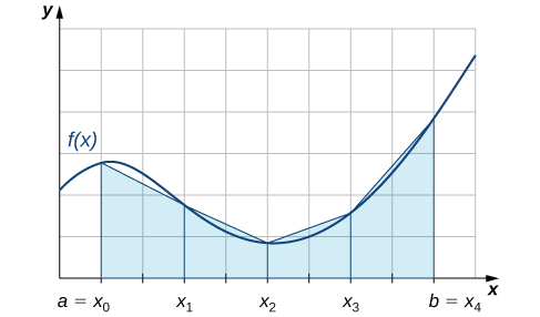
The trapezoidal rule for estimating definite integrals uses trapezoids rather than rectangles to approximate the area under a curve. To gain insight into the final form of the rule, consider the trapezoids shown in Figure 3.14. We assume that the length of each subinterval is given by $Δ x .$ First, recall that the area of a trapezoid with a height of h and bases of length $b_{1}$ and $b_{2}$ is given by $Area = \frac{1}{2} h (b_{1} + b_{2}) .$ We see that the first trapezoid has a height $Δ x$ and parallel bases of length $f (x_{0})$ and $f (x_{1}) .$ Thus, the area of the first trapezoid in Figure 3.14 is

\frac{1}{2} Δ x (f (x_{0}) + f (x_{1})) .

The areas of the remaining three trapezoids are

\frac{1}{2} Δ x (f (x_{1}) + f (x_{2})), \frac{1}{2} Δ x (f (x_{2}) + f (x_{3})), and \frac{1}{2} Δ x (f (x_{3}) + f (x_{4})) .

Consequently,

\int_{a}^{b} f (x) d x \approx \frac{1}{2} Δ x (f (x_{0}) + f (x_{1})) + \frac{1}{2} Δ x (f (x_{1}) + f (x_{2})) + \frac{1}{2} Δ x (f (x_{2}) + f (x_{3})) + \frac{1}{2} Δ x (f (x_{3}) + f (x_{4})) .

After taking out a common factor of $\frac{1}{2} Δ x$ and combining like terms, we have

\int_{a}^{b} f (x) d x \approx \frac{1}{2} Δ x (f (x_{0}) + 2 f (x_{1}) + 2 f (x_{2}) + 2 f (x_{3}) + f (x_{4})) .

Generalizing, we formally state the following rule.

The Trapezoidal Rule

Assume that $f (x)$ is continuous over $[a, b] .$ Let n be a positive integer and $Δ x = \frac{b - a}{n} .$ Let $[a, b]$ be divided into $n$ subintervals, each of length $Δ x,$ with endpoints at $P = {x_{0}, x_{1}, x_{2} …, x_{n}} .$ Set

T_{n} = \frac{1}{2} Δ x (f (x_{0}) + 2 f (x_{1}) + 2 f (x_{2}) + \dots + 2 f (x_{n - 1}) + f (x_{n})) .

3.11

Then, $lim_{n \to + \infty} T_{n} = \int_{a}^{b} f (x) d x .$

Before continuing, let’s make a few observations about the trapezoidal rule. First of all, it is useful to note that

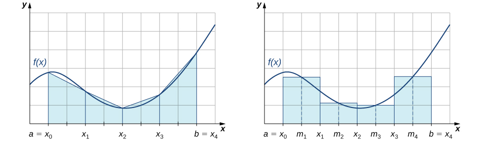
T_{n} = \frac{1}{2} (L_{n} + R_{n}) where L_{n} = \sum_{i = 1}^{n} f (x_{i - 1}) Δ x and R_{n} = \sum_{i = 1}^{n} f (x_{i}) Δ x .

That is, $L_{n}$ and $R_{n}$ approximate the integral using the left-hand and right-hand endpoints of each subinterval, respectively. In addition, a careful examination of Figure 3.15 leads us to make the following observations about using the trapezoidal rules and midpoint rules to estimate the definite integral of a nonnegative function. The trapezoidal rule tends to overestimate the value of a definite integral systematically over intervals where the function is concave up and to underestimate the value of a definite integral systematically over intervals where the function is concave down. On the other hand, the midpoint rule tends to average out these errors somewhat by partially overestimating and partially underestimating the value of the definite integral over these same types of intervals. This leads us to hypothesize that, in general, the midpoint rule tends to be more accurate than the trapezoidal rule.

This figure has two graphs, both of the same non-negative function in the first quadrant. The function increases and decreases. The quadrant is divided into a grid. The first graph, beginning on the x-axis at the point labeled a = x sub 0, there are trapezoids shaded whose heights are approximately the height of the curve. The x-axis is scaled by increments of a = x sub 0, xsub1, x sub 2, x sub 3, and b = x sub 4. The second graph has on the x-axis at the point labeled a = x sub 0. There are rectangles shaded whose heights are approximately the height of the curve. The x-axis is scaled by increments of m sub 1, x sub 1, m sub 2, x sub 2, m sub 3, x sub 3, m sub 4 and b = x sub 4. — Figure 3.15 The trapezoidal rule tends to be less accurate than the midpoint rule.

Using the Trapezoidal Rule

Use the trapezoidal rule to estimate $\int_{0}^{1} x^{2} d x$ using four subintervals.

The endpoints of the subintervals consist of elements of the set $P = {0, \frac{1}{4}, \frac{1}{2}, \frac{3}{4}, 1}$ and $Δ x = \frac{1 - 0}{4} = \frac{1}{4} .$ Thus,

\begin{matrix} \int_{0}^{1} x^{2} d x & \approx \frac{1}{2} \cdot \frac{1}{4} (f (0) + 2 f (\frac{1}{4}) + 2 f (\frac{1}{2}) + 2 f (\frac{3}{4}) + f (1)) \\ = \frac{1}{8} (0 + 2 \cdot \frac{1}{16} + 2 \cdot \frac{1}{4} + 2 \cdot \frac{9}{16} + 1) \\ = \frac{11}{32} . \end{matrix}

Use the trapezoidal rule with $n = 2$ to estimate $\int_{1}^{2} \frac{1}{x} d x .$

$\frac{17}{24}$

Hint

Set $Δ x = \frac{1}{2} .$ The endpoints of the subintervals are the elements of the set $P = {1, \frac{3}{2}, 2} .$

Absolute and Relative Error

An important aspect of using these numerical approximation rules consists of calculating the error in using them for estimating the value of a definite integral. We first need to define absolute error and relative error.

Definition

If $B$ is our estimate of some quantity having an actual value of $A,$ then the absolute error is given by $| A - B | .$ The relative error is the error as a percentage of the absolute value and is given by $| \frac{A - B}{A} | = | \frac{A - B}{A} | \cdot 100 % .$

Calculating Error in the Midpoint Rule

Calculate the absolute and relative error in the estimate of $\int_{0}^{1} x^{2} d x$ using the midpoint rule, found in Example 3.39.

The calculated value is $\int_{0}^{1} x^{2} d x = \frac{1}{3}$ and our estimate from the example is $M_{4} = \frac{21}{64} .$ Thus, the absolute error is given by $| (\frac{1}{3}) - (\frac{21}{64}) | = \frac{1}{192} \approx 0.0052 .$ The relative error is

\frac{1 / 192}{1 / 3} = \frac{1}{64} \approx 0.015625 \approx 1.6 % .

Calculating Error in the Trapezoidal Rule

Calculate the absolute and relative error in the estimate of $\int_{0}^{1} x^{2} d x$ using the trapezoidal rule, found in Example 3.41.

The calculated value is $\int_{0}^{1} x^{2} d x = \frac{1}{3}$ and our estimate from the example is $T_{4} = \frac{11}{32} .$ Thus, the absolute error is given by $| \frac{1}{3} - \frac{11}{32} | = \frac{1}{96} \approx 0.0104 .$ The relative error is given by

\frac{1 / 96}{1 / 3} = 0.03125 \approx 3.1 % .

In an earlier checkpoint, we estimated $\int_{1}^{2} \frac{1}{x} d x$ to be $\frac{24}{35}$ using $T_{2} .$ The actual value of this integral is $ln 2 .$ Using $\frac{24}{35} \approx 0.6857$ and $ln 2 \approx 0.6931,$ calculate the absolute error and the relative error.

0.0074, 1.1%

Hint

Use the previous examples as a guide.

In the two previous examples, we were able to compare our estimate of an integral with the actual value of the integral; however, we do not typically have this luxury. In general, if we are approximating an integral, we are doing so because we cannot compute the exact value of the integral itself easily. Therefore, it is often helpful to be able to determine an upper bound for the error in an approximation of an integral. The following theorem provides error bounds for the midpoint and trapezoidal rules. The theorem is stated without proof.

Error Bounds for the Midpoint and Trapezoidal Rules

Let $f (x)$ be a continuous function over $[a, b],$ having a second derivative $f^{″} (x)$ over this interval. If $M$ is the maximum value of $| f^{″} (x) |$ over $[a, b],$ then the upper bounds for the error in using $M_{n}$ and $T_{n}$ to estimate $\int_{a}^{b} f (x) d x$ are

Error in M_{n} \leq \frac{M {(b - a)}^{3}}{24 n^{2}}

3.12

and

Error in T_{n} \leq \frac{M {(b - a)}^{3}}{12 n^{2}} .

3.13

We can use these bounds to determine the value of $n$ necessary to guarantee that the error in an estimate is less than a specified value.

Determining the Number of Intervals to Use

What value of $n$ should be used to guarantee that an estimate of $\int_{0}^{1} e^{x^{2}} d x$ is accurate to within 0.01 if we use the midpoint rule?

We begin by determining the value of $M,$ the maximum value of $| f^{″} (x) |$ over $[0, 1]$ for $f (x) = e^{x^{2}} .$ Since $f^{'} (x) = 2 x e^{x^{2}},$ we have

f^{″} (x) = 2 e^{x^{2}} + 4 x^{2} e^{x^{2}} .

Thus,

| f^{″} (x) | = 2 e^{x^{2}} (1 + 2 x^{2}) \leq 2 \cdot e \cdot 3 = 6 e .

From the error-bound Equation 3.12, we have

Error in M_{n} \leq \frac{M {(b - a)}^{3}}{24 n^{2}} \leq \frac{6 e {(1 - 0)}^{3}}{24 n^{2}} = \frac{6 e}{24 n^{2}} .

Now we solve the following inequality for $n :$

\frac{6 e}{24 n^{2}} \leq 0.01 .

Thus, $n \geq \sqrt{\frac{600 e}{24}} \approx 8.24 .$ Since $n$ must be an integer satisfying this inequality, a choice of $n = 9$ would guarantee that $| \int_{0}^{1} e^{x^{2}} d x - M_{n} | < 0.01 .$

Analysis

We might have been tempted to round $8.24$ down and choose $n = 8,$ but this would be incorrect because we must have an integer greater than or equal to $8.24 .$ We need to keep in mind that the error estimates provide an upper bound only for the error. The actual estimate may, in fact, be a much better approximation than is indicated by the error bound.

Use Equation 3.13 to find an upper bound for the error in using $M_{4}$ to estimate $\int_{0}^{1} x^{2} d x .$

$\frac{1}{192}$

Hint

$f^{″} (x) = 2,$ so $M = 2 .$

Simpson’s Rule

With the midpoint rule, we estimated areas of regions under curves by using rectangles. In a sense, we approximated the curve with piecewise constant functions. With the trapezoidal rule, we approximated the curve by using piecewise linear functions. What if we were, instead, to approximate a curve using piecewise quadratic functions? With Simpson’s rule, we do just this. We partition the interval into an even number of subintervals, each of equal width. Over the first pair of subintervals we approximate $\int_{x_{0}}^{x_{2}} f (x) d x$ with $\int_{x_{0}}^{x_{2}} p (x) d x,$ where $p (x) = A x^{2} + B x + C$ is the quadratic function passing through $(x_{0}, f (x_{0})),$ $(x_{1}, f (x_{1})),$ and $(x_{2}, f (x_{2}))$ (Figure 3.16). Over the next pair of subintervals we approximate $\int_{x_{2}}^{x_{4}} f (x) d x$ with the integral of another quadratic function passing through $(x_{2}, f (x_{2})),$ $(x_{3}, f (x_{3})),$ and $(x_{4}, f (x_{4})) .$ This process is continued with each successive pair of subintervals.

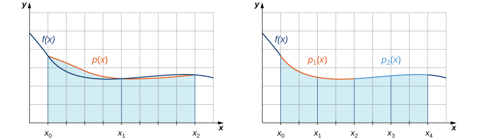
To understand the formula that we obtain for Simpson’s rule, we begin by deriving a formula for this approximation over the first two subintervals. As we go through the derivation, we need to keep in mind the following relationships:

\begin{matrix} f (x_{0}) = p (x_{0}) = A x_{0}^{2} + B x_{0} + C \\ f (x_{1}) = p (x_{1}) = A x_{1}^{2} + B x_{1} + C \\ f (x_{2}) = p (x_{2}) = A x_{2}^{2} + B x_{2} + C \end{matrix}

$x_{2} - x_{0} = 2 Δ x,$ where $Δ x$ is the length of a subinterval.

x_{2} + x_{0} = 2 x_{1}, since x_{1} = \frac{(x_{2} + x_{0})}{2} .

Thus,

\begin{matrix} \int_{x_{0}}^{x_{2}} f (x) d x & \approx \int_{x_{0}}^{x_{2}} p (x) d x \\ = \int_{x_{0}}^{x_{2}} (A x^{2} + B x + C) d x \\ = \frac{A}{3} x^{3} + \frac{B}{2} x^{2} + C x | \begin{matrix} ^{x_{2}} \\ _{x_{0}} \end{matrix} & Find the antiderivative. \\ = \frac{A}{3} (x_{2}^{3} - x_{0}^{3}) + \frac{B}{2} (x_{2}^{2} - x_{0}^{2}) + C (x_{2} - x_{0}) & Evaluate the antiderivative. \\ = \frac{A}{3} (x_{2} - x_{0}) (x_{2}^{2} + x_{2} x_{0} + x_{0}^{2}) \\ + \frac{B}{2} (x_{2} - x_{0}) (x_{2} + x_{0}) + C (x_{2} - x_{0}) \\ = \frac{x_{2} - x_{0}}{6} (2 A (x_{2}^{2} + x_{2} x_{0} + x_{0}^{2}) + 3 B (x_{2} + x_{0}) + 6 C) & Factor out \frac{x_{2} - x_{0}}{6} . \\ = \frac{Δ x}{3} ((A x_{2}^{2} + B x_{2} + C) + (A x_{0}^{2} + B x_{0} + C) \\ + A (x_{2}^{2} + 2 x_{2} x_{0} + x_{0}^{2}) + 2 B (x_{2} + x_{0}) + 4 C) \\ = \frac{Δ x}{3} (f (x_{2}) + f (x_{0}) + A {(x_{2} + x_{0})}^{2} + 2 B (x_{2} + x_{0}) + 4 C) & Rearrange the terms. \\ \begin{matrix} Factor and substitute. \\ f (x_{2}) = A x_{2}^{2} + B x_{2} + C and \\ f (x_{0}) = A x_{0}^{2} + B x_{0} + C . \end{matrix} \\ = \frac{Δ x}{3} (f (x_{2}) + f (x_{0}) + A {(2 x_{1})}^{2} + 2 B (2 x_{1}) + 4 C) & Substitute x_{2} + x_{0} = 2 x_{1} . \\ = \frac{Δ x}{3} (f (x_{2}) + 4 f (x_{1}) + f (x_{0})) . & \begin{matrix} Expand and substitute \\ f (x_{1}) = A x_{1}^{2} + B x_{1} + C . \end{matrix} \end{matrix}

If we approximate $\int_{x_{2}}^{x_{4}} f (x) d x$ using the same method, we see that we have

\int_{x_{2}}^{x_{4}} f (x) d x \approx \frac{Δ x}{3} (f (x_{4}) + 4 f (x_{3}) + f (x_{2})) .

Combining these two approximations, we get

\int_{x_{2}}^{x_{4}} f (x) d x = \frac{Δ x}{3} (f (x_{0}) + 4 f (x_{1}) + 2 f (x_{2}) + 4 f (x_{3}) + f (x_{4})) .

The pattern continues as we add pairs of subintervals to our approximation. The general rule may be stated as follows.

Simpson’s Rule

Assume that $f (x)$ is continuous over $[a, b] .$ Let n be a positive even integer and $Δ x = \frac{b - a}{n} .$ Let $[a, b]$ be divided into $n$ subintervals, each of length $Δ x,$ with endpoints at $P = {x_{0}, x_{1}, x_{2},…, x_{n}} .$ Set

S_{n} = \frac{Δ x}{3} (f (x_{0}) + 4 f (x_{1}) + 2 f (x_{2}) + 4 f (x_{3}) + 2 f (x_{4}) + \dots + 2 f (x_{n - 2}) + 4 f (x_{n - 1}) + f (x_{n})) .

3.14

Then,

lim_{n \to + \infty} S_{n} = \int_{a}^{b} f (x) d x .

Just as the trapezoidal rule is the average of the left-hand and right-hand rules for estimating definite integrals, Simpson’s rule may be obtained from the midpoint and trapezoidal rules by using a weighted average. It can be shown that $S_{2 n} = (\frac{2}{3}) M_{n} + (\frac{1}{3}) T_{n} .$

It is also possible to put a bound on the error when using Simpson’s rule to approximate a definite integral. The bound in the error is given by the following rule:

Rule: Error Bound for Simpson’s Rule

Let $f (x)$ be a continuous function over $[a, b]$ having a fourth derivative, $f^{(4)} (x),$ over this interval. If $M$ is the maximum value of $| f^{(4)} (x) |$ over $[a, b],$ then the upper bound for the error in using $S_{n}$ to estimate $\int_{a}^{b} f (x) d x$ is given by

Error in S_{n} \leq \frac{M {(b - a)}^{5}}{180 n^{4}} .

3.15

Applying Simpson’s Rule 1

Use $S_{2}$ to approximate $\int_{0}^{1} x^{3} d x .$ Estimate a bound for the error in $S_{2} .$

Since $[0, 1]$ is divided into two intervals, each subinterval has length $Δ x = \frac{1 - 0}{2} = \frac{1}{2} .$ The endpoints of these subintervals are ${0, \frac{1}{2}, 1} .$ If we set $f (x) = x^{3},$ then

$S_{4} = \frac{1}{3} \cdot \frac{1}{2} (f (0) + 4 f (\frac{1}{2}) + f (1)) = \frac{1}{6} (0 + 4 \cdot \frac{1}{8} + 1) = \frac{1}{4} .$ Since $f^{(4)} (x) = 0$ and consequently $M = 0,$ we see that

Error in S_{2} \leq \frac{0 {(1)}^{5}}{180 \cdot 2^{4}} = 0 .

This bound indicates that the value obtained through Simpson’s rule is exact. A quick check will verify that, in fact, $\int_{0}^{1} x^{3} d x = \frac{1}{4} .$

Applying Simpson’s Rule 2

Use $S_{6}$ to estimate the length of the curve $y = \frac{1}{2} x^{2}$ over $[1, 4] .$

The length of $y = \frac{1}{2} x^{2}$ over $[1, 4]$ is $\int_{1}^{4} \sqrt{1 + x^{2}} d x .$ If we divide $[1, 4]$ into six subintervals, then each subinterval has length $Δ x = \frac{4 - 1}{6} = \frac{1}{2},$ and the endpoints of the subintervals are ${1, \frac{3}{2}, 2, \frac{5}{2}, 3, \frac{7}{2}, 4} .$ Setting $f (x) = \sqrt{1 + x^{2}},$

S_{6} = \frac{1}{3} \cdot \frac{1}{2} (f (1) + 4 f (\frac{3}{2}) + 2 f (2) + 4 f (\frac{5}{2}) + 2 f (3) + 4 f (\frac{7}{2}) + f (4)) .

After substituting, we have

\begin{matrix} S_{6} & = \frac{1}{6} (1.4142 + 4 \cdot 1.80278 + 2 \cdot 2.23607 + 4 \cdot 2.69258 + 2 \cdot 3.16228 + 4 \cdot 3.64005 + 4.12311) \\ \approx 8.14594. \end{matrix}

Use $S_{2}$ to estimate $\int_{1}^{2} \frac{1}{x} d x .$

$\frac{25}{36}$

Hint

$S_{2} = (\frac{1}{3} Δ x (f (x_{0}) + 4 f (x_{1}) + f (x_{2}))$

Key Concepts

We can use numerical integration to estimate the values of definite integrals when a closed form of the integral is difficult to find or when an approximate value only of the definite integral is needed.
The most commonly used techniques for numerical integration are the midpoint rule, trapezoidal rule, and Simpson’s rule.
The midpoint rule approximates the definite integral using rectangular regions whereas the trapezoidal rule approximates the definite integral using trapezoidal approximations.
Simpson’s rule approximates the definite integral by first approximating the original function using piecewise quadratic functions.

Key Equations

Midpoint rule	$M_{n} = \sum_{i = 1}^{n} f (m_{i}) Δ x$
Trapezoidal rule	$T_{n} = \frac{1}{2} Δ x (f (x_{0}) + 2 f (x_{1}) + 2 f (x_{2}) + \dots + 2 f (x_{n - 1}) + f (x_{n}))$
Simpson’s rule	$S_{n} = \frac{Δ x}{3} (f (x_{0}) + 4 f (x_{1}) + 2 f (x_{2}) + 4 f (x_{3}) + 2 f (x_{4}) + 4 f (x_{5}) + \dots + 2 f (x_{n - 2}) + 4 f (x_{n - 1}) + f (x_{n}))$
Error bound for midpoint rule	$Error in M_{n} \leq \frac{M {(b - a)}^{3}}{24 n^{2}}$
Error bound for trapezoidal rule	$Error in T_{n} \leq \frac{M {(b - a)}^{3}}{12 n^{2}}$
Error bound for Simpson’s rule	$Error in S_{n} \leq \frac{M {(b - a)}^{5}}{180 n^{4}}$

Approximate the following integrals using either the midpoint rule, trapezoidal rule, or Simpson’s rule as indicated. (Round answers to three decimal places.)

$\int_{1}^{2} \frac{d x}{x};$ trapezoidal rule; $n = 5$

0.696

$\int_{0}^{3} \sqrt{4 + x^{3}} d x;$ trapezoidal rule; $n = 6$

$\int_{0}^{3} \sqrt{4 + x^{3}} d x;$ trapezoidal rule; $n = 3$

9.484

$\int_{0}^{12} x^{2} d x;$ midpoint rule; $n = 6$

$\int_{0}^{1} {sin}^{2} (π x) d x;$ midpoint rule; $n = 3$

0.5000

Use the midpoint rule with eight subdivisions to estimate $\int_{2}^{4} x^{2} d x .$

Use the trapezoidal rule with four subdivisions to estimate $\int_{2}^{4} x^{2} d x .$

$T_{4} = 18.75$

Find the exact value of $\int_{2}^{4} x^{2} d x .$ Find the error of approximation between the exact value and the value calculated using the trapezoidal rule with four subdivisions. Draw a graph to illustrate.

Approximate the integral to three decimal places using the indicated rule.

$\int_{0}^{1} {sin}^{2} (π x) d x;$ trapezoidal rule; $n = 6$

0.500

$\int_{0}^{3} \frac{1}{1 + x^{3}} d x;$ trapezoidal rule; $n = 6$

$\int_{0}^{3} \frac{1}{1 + x^{3}} d x;$ trapezoidal rule; $n = 3$

1.129

$\int_{0}^{0.8} e^{− x^{2}} d x;$ trapezoidal rule; $n = 4$

$\int_{0}^{0.8} e^{− x^{2}} d x;$ Simpson’s rule; $n = 4$

0.6577

$\int_{0}^{0.4} sin (x^{2}) d x;$ trapezoidal rule; $n = 4$

$\int_{0}^{0.4} sin (x^{2}) d x;$ Simpson’s rule; $n = 4$

0.0213

$\int_{0.1}^{0.5} \frac{cos x}{x} d x;$ trapezoidal rule; $n = 4$

$\int_{0.1}^{0.5} \frac{cos x}{x} d x;$ Simpson’s rule; $n = 4$

1.5629

Evaluate $\int_{0}^{1} \frac{d x}{1 + x^{2}}$ exactly and show that the result is $π / 4 .$ Then, find the approximate value of the integral using the trapezoidal rule with $n = 4$ subdivisions. Use the result to approximate the value of $π .$

Approximate $\int_{2}^{4} \frac{1}{ln x} d x$ using the midpoint rule with four subdivisions to four decimal places.

1.9133

Approximate $\int_{2}^{4} \frac{1}{ln x} d x$ using the trapezoidal rule with eight subdivisions to four decimal places.

Use the trapezoidal rule with four subdivisions to estimate $\int_{0}^{0.8} x^{3} d x$ to four decimal places.

$T(4) = 0.1088$

Use the trapezoidal rule with four subdivisions to estimate $\int_{0}^{0.8} x^{3} d x .$ Compare this value with the exact value and find the error estimate.

Using Simpson’s rule with four subdivisions, find $\int_{0}^{π / 2} cos (x) d x .$

1.0

Show that the exact value of $\int_{0}^{1} x e^{− x} d x = 1 - \frac{2}{e} .$ Find the absolute error if you approximate the integral using the midpoint rule with 16 subdivisions.

Given $\int_{0}^{1} x e^{− x} d x = 1 - \frac{2}{e},$ use the trapezoidal rule with 16 subdivisions to approximate the integral and find the absolute error.

Approximate error is 0.000325.

Find an upper bound for the error in estimating $\int_{0}^{3} (5 x + 4) d x$ using the trapezoidal rule with six steps.

Find an upper bound for the error in estimating $\int_{4}^{5} \frac{1}{{(x - 1)}^{2}} d x$ using the trapezoidal rule with seven subdivisions.

$\frac{1}{7938}$

Find an upper bound for the error in estimating $\int_{0}^{3} (6 x^{2} - 1) d x$ using Simpson’s rule with $n = 10$ steps.

Find an upper bound for the error in estimating $\int_{2}^{5} \frac{1}{x - 1} d x$ using Simpson’s rule with $n = 10$ steps.

$\frac{81}{25, 000}$

Find an upper bound for the error in estimating $\int_{0}^{π} 2 x cos (x) d x$ using Simpson’s rule with four steps.

Estimate the minimum number of subintervals needed to approximate the integral $\int_{1}^{4} (5 x^{2} + 8) d x$ with an error magnitude of less than 0.0001 using the trapezoidal rule.

475

Determine a value of n such that the trapezoidal rule will approximate $\int_{0}^{1} \sqrt{1 + x^{2}} d x$ with an error of no more than 0.01.

Estimate the minimum number of subintervals needed to approximate the integral $\int_{2}^{3} (2 x^{3} + 4 x) d x$ with an error of magnitude less than 0.0001 using the trapezoidal rule.

174

Estimate the minimum number of subintervals needed to approximate the integral $\int_{3}^{4} \frac{1}{{(x - 1)}^{2}} d x$ with an error magnitude of less than 0.0001 using the trapezoidal rule.

Use Simpson’s rule with four subdivisions to approximate the area under the probability density function $y = \frac{1}{\sqrt{2 π}} e^{− x^{2} / 2}$ from $x = 0$ to $x = 0.4 .$

0.1544

Use Simpson’s rule with $n = 14$ to approximate (to three decimal places) the area of the region bounded by the graphs of $y = 0,$ $x = 0,$ and $x = π / 2 .$

The length of one arch of the curve $y = 3 sin (2 x)$ is given by $L = \int_{0}^{π / 2} \sqrt{1 + 36 {cos}^{2} (2 x)} d x .$ Estimate L using the trapezoidal rule with $n = 6 .$

6.2807

The length of the ellipse $x = a cos (t), y = b sin (t), 0 \leq t \leq 2 π$ is given by $L = 4 a \int_{0}^{π / 2} \sqrt{1 - e^{2} {cos}^{2} (t)} d t,$ where e is the eccentricity of the ellipse. Use Simpson’s rule with $n = 6$ subdivisions to estimate the length of the ellipse when $a = 2$ and $e = 1 / 3 .$

Estimate the area of the surface generated by revolving the curve $y = cos (2 x), 0 \leq x \leq \frac{π}{4}$ about the x-axis. Use the trapezoidal rule with six subdivisions.

4.606

Estimate the area of the surface generated by revolving the curve $y = 2 x^{2},$ $0 \leq x \leq 3$ about the x-axis. Use Simpson’s rule with $n = 6 .$

The growth rate of a certain tree (in feet) is given by $y = \frac{2}{t + 1} + e^{− t^{2} / 2},$ where t is time in years. Estimate the growth of the tree through the end of the second year by using Simpson’s rule, using two subintervals. (Round the answer to the nearest hundredth.)

3.41 ft

[T] Use a calculator to approximate $\int_{0}^{1} sin (π x) d x$ using the midpoint rule with 25 subdivisions. Compute the relative error of approximation.

[T] Given $\int_{1}^{5} (3 x^{2} - 2 x) d x = 100,$ approximate the value of this integral using the trapezoidal rule with 16 subdivisions and determine the absolute error.

$T_{16} = 100.125;$ absolute error = 0.125

Given that we know the Fundamental Theorem of Calculus, why would we want to develop numerical methods for definite integrals?

The table represents the coordinates $(x, y)$ that give the boundary of a lot. The units of measurement are meters. Use the trapezoidal rule to estimate the number of square meters of land that is in this lot.

x	y	x	y
0	125	600	95
100	125	700	88
200	120	800	75
300	112	900	35
400	90	1000	0
500	90

about 89,250 m²

Choose the correct answer. When Simpson’s rule is used to approximate the definite integral, it is necessary that the number of partitions be____

an even number
odd number
either an even or an odd number
a multiple of 4

The “Simpson” sum is based on the area under a ____.

parabola

The error formula for Simpson’s rule depends on___.

$f (x)$
$f^{'} (x)$
$f^{(4)} (x)$
the number of steps

Glossary

absolute error: if $B$ is an estimate of some quantity having an actual value of $A,$ then the absolute error is given by $| A - B |$
midpoint rule: a rule that uses a Riemann sum of the form $M_{n} = \sum_{i = 1}^{n} f (m_{i}) Δ x,$ where $m_{i}$ is the midpoint of the ith subinterval to approximate $\int_{a}^{b} f (x) d x$
numerical integration: the variety of numerical methods used to estimate the value of a definite integral, including the midpoint rule, trapezoidal rule, and Simpson’s rule
relative error: error as a percentage of the absolute value, given by $| \frac{A - B}{A} | = | \frac{A - B}{A} | \cdot 100 %$
Simpson’s rule: a rule that approximates $\int_{a}^{b} f (x) d x$ using the integrals of a piecewise quadratic function. The approximation $S_{n}$ to $\int_{a}^{b} f (x) d x$ is given by $S_{n} = \frac{Δ x}{3} (\begin{matrix} f (x_{0}) + 4 f (x_{1}) + 2 f (x_{2}) + 4 f (x_{3}) + 2 f (x_{4}) + 4 f (x_{5}) \\ + \dots + 2 f (x_{n - 2}) + 4 f (x_{n - 1}) + f (x_{n}) \end{matrix})$ trapezoidal rule a rule that approximates $\int_{a}^{b} f (x) d x$ using trapezoids