3.9 Derivatives of Exponential and Logarithmic Functions

Find the derivative of exponential functions.
Find the derivative of logarithmic functions.
Use logarithmic differentiation to determine the derivative of a function.

So far, we have learned how to differentiate a variety of functions, including trigonometric, inverse, and implicit functions. In this section, we explore derivatives of exponential and logarithmic functions. As we discussed in Introduction to Functions and Graphs, exponential functions play an important role in modeling population growth and the decay of radioactive materials. Logarithmic functions can help rescale large quantities and are particularly helpful for rewriting complicated expressions.

Derivative of the Exponential Function

Just as when we found the derivatives of other functions, we can find the derivatives of exponential and logarithmic functions using formulas. As we develop these formulas, we need to make certain basic assumptions. The proofs that these assumptions hold are beyond the scope of this course.

First of all, we begin with the assumption that the function $B (x) = b^{x}, b > 0,$ is defined for every real number and is continuous. In previous courses, the values of exponential functions for all rational numbers were defined—beginning with the definition of $b^{n},$ where $n$ is a positive integer—as the product of $b$ multiplied by itself $n$ times. Later, we defined $b^{0} = 1, b^{− n} = \frac{1}{b^{n}},$ for a positive integer $n,$ and $b^{s / t} = (\sqrt[t]{b})^{s}$ for positive integers $s$ and $t .$ These definitions leave open the question of the value of $b^{r}$ where $r$ is an arbitrary real number. By assuming the continuity of $B (x) = b^{x}, b > 0,$ we may interpret $b^{r}$ as $lim_{x \to r} b^{x}$ where the values of $x$ as we take the limit are rational. For example, we may view $4^{π}$ as the number satisfying

\begin{array}{l} 4^{3} < 4^{π} < 4^{4}, 4^{3.1} < 4^{π} < 4^{3.2}, 4^{3.14} < 4^{π} < 4^{3.15}, \\ 4^{3.141} < 4^{π} < 4^{3.142}, 4^{3.1415} < 4^{π} < 4^{3.1416}, … . \end{array}

As we see in the following table, $4^{π} \approx 77.88 .$

Table 3.6 Approximating a Value of $4^{π}$
$x$	$4^{x}$	$x$	$4^{x}$
$3$	64	$3.141593$	77.8802710486
$3.1$	73.5166947198	$3.1416$	77.8810268071
$3.14$	77.7084726013	$3.142$	77.9242251944
$3.141$	77.8162741237	$3.15$	78.7932424541
$3.1415$	77.8702309526	$3.2$	84.4485062895
$3.14159$	77.8799471543	$4$	256

We also assume that for $B (x) = b^{x}, b > 0,$ the value $B^{'} (0)$ of the derivative exists. In this section, we show that by making this one additional assumption, it is possible to prove that the function $B (x)$ is differentiable everywhere.

We make one final assumption: that there is a unique value of $b > 0$ for which $B^{'} (0) = 1 .$ We define $e$ to be this unique value, as we did in Introduction to Functions and Graphs. Figure 3.33 provides graphs of the functions $y = 2^{x}, y = 3^{x}, y = {2.7}^{x},$ and $y = {2.8}^{x} .$ A visual estimate of the slopes of the tangent lines to these functions at 0 provides evidence that the value of e lies somewhere between 2.7 and 2.8. The function $E (x) = e^{x}$ is called the natural exponential function. Its inverse, $L (x) = {log}_{e} x = ln x$ is called the natural logarithmic function.

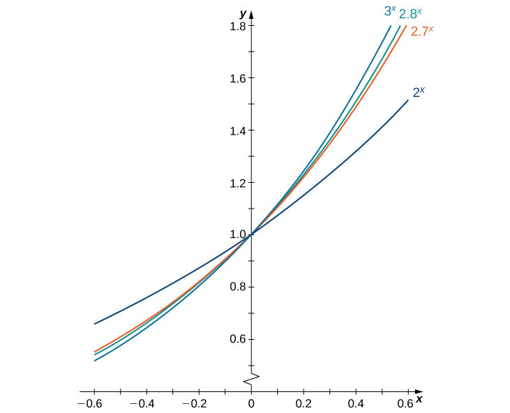
The graphs of 3x, 2.8x, 2.7x, and 2x are shown. In quadrant I, their order from least to greatest is 2x, 2.7x, 2.8x, and 3x. In quadrant II, this order is reversed. All cross the y-axis at (0, 1). — Figure 3.33 The graph of $E (x) = e^{x}$ is between $y = 2^{x}$ and $y = 3^{x} .$

For a better estimate of $e,$ we may construct a table of estimates of $B^{'} (0)$ for functions of the form $B (x) = b^{x} .$ Before doing this, recall that

B^{'} (0) = lim_{x \to 0} \frac{b^{x} - b^{0}}{x - 0} = lim_{x \to 0} \frac{b^{x} - 1}{x} \approx \frac{b^{x} - 1}{x}

for values of $x$ very close to zero. For our estimates, we choose $x = 0.00001$ and $x = −0.00001$ to obtain the estimate

\frac{b^{−0.00001} - 1}{−0.00001} < B^{'} (0) < \frac{b^{0.00001} - 1}{0.00001} .

See the following table.

Table 3.7 Estimating a Value of $e$
$b$	$\frac{b^{−0.00001} - 1}{−0.00001} < B^{'} (0) < \frac{b^{0.00001} - 1}{0.00001}$	$b$	$\frac{b^{−0.00001} - 1}{−0.00001} < B^{'} (0) < \frac{b^{0.00001} - 1}{0.00001}$
$2$	$0.693145 < B^{'} (0) < 0.69315$	$2.7183$	$1.000002 < B^{'} (0) < 1.000012$
$2.7$	$0.993247 < B^{'} (0) < 0.993257$	$2.719$	$1.000259 < B^{'} (0) < 1.000269$
$2.71$	$0.996944 < B^{'} (0) < 0.996954$	$2.72$	$1.000627 < B^{'} (0) < 1.000637$
$2.718$	$0.999891 < B^{'} (0) < 0.999901$	$2.8$	$1.029614 < B^{'} (0) < 1.029625$
$2.7182$	$0.999965 < B^{'} (0) < 0.999975$	$3$	$1.098606 < B^{'} (0) < 1.098618$

The evidence from the table suggests that $2.7182 < e < 2.7183 .$

The graph of $E (x) = e^{x}$ together with the line $y = x + 1$ are shown in Figure 3.34. This line is tangent to the graph of $E (x) = e^{x}$ at $x = 0 .$

Graph of the function ex along with its tangent at (0, 1), x + 1. — Figure 3.34 The tangent line to $E (x) = e^{x}$ at $x = 0$ has slope 1.

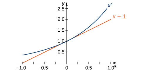
Now that we have laid out our basic assumptions, we begin our investigation by exploring the derivative of $B (x) = b^{x}, b > 0 .$ Recall that we have assumed that $B^{'} (0)$ exists. By applying the limit definition to the derivative we conclude that

B^{'} (0) = lim_{h \to 0} \frac{b^{0 + h} - b^{0}}{h} = lim_{h \to 0} \frac{b^{h} - 1}{h} .

3.28

Turning to $B^{'} (x),$ we obtain the following.

\begin{matrix} B^{'} (x) & = lim_{h \to 0} \frac{b^{x + h} - b^{x}}{h} & Apply the limit definition of the derivative. \\ = lim_{h \to 0} \frac{b^{x} b^{h} - b^{x}}{h} & Note that b^{x + h} = b^{x} b^{h} . \\ = lim_{h \to 0} \frac{b^{x} (b^{h} - 1)}{h} & Factor out b^{x} . \\ = b^{x} lim_{h \to 0} \frac{b^{h} - 1}{h} & Apply a property of limits. \\ = b^{x} B^{'} (0) & Use B^{'} (0) = lim_{h \to 0} \frac{b^{0 + h} - b^{0}}{h} = lim_{h \to 0} \frac{b^{h} - 1}{h} . \end{matrix}

We see that on the basis of the assumption that $B (x) = b^{x}$ is differentiable at $0, B (x)$ is not only differentiable everywhere, but its derivative is

B^{'} (x) = b^{x} B^{'} (0) .

3.29

For $E (x) = e^{x}, E^{'} (0) = 1 .$ Thus, we have $E^{'} (x) = e^{x} .$ (The value of $B^{'} (0)$ for an arbitrary function of the form $B (x) = b^{x}, b > 0,$ will be derived later.)

Derivative of the Natural Exponential Function

Let $E (x) = e^{x}$ be the natural exponential function. Then

E^{'} (x) = e^{x} .

In general,

\frac{d}{d x} (e^{g (x)}) = e^{g (x)} g^{'} (x) .

Derivative of an Exponential Function

Find the derivative of $f (x) = e^{tan (2 x)} .$

Using the derivative formula and the chain rule,

\begin{matrix} f^{'} (x) & = e^{tan (2 x)} \frac{d}{d x} (tan (2 x)) \\ = e^{tan (2 x)} {sec}^{2} (2 x) \cdot 2 . \end{matrix}

Combining Differentiation Rules

Find the derivative of $y = \frac{e^{x^{2}}}{x} .$

Use the derivative of the natural exponential function, the quotient rule, and the chain rule.

\begin{matrix} y^{'} & = \frac{(e^{x^{2}} \cdot 2) x \cdot x - 1 \cdot e^{x^{2}}}{x^{2}} & Apply the quotient rule. \\ = \frac{e^{x^{2}} (2 x^{2} - 1)}{x^{2}} & Simplify. \end{matrix}

Find the derivative of $h (x) = x e^{2 x} .$

$h^{'} (x) = e^{2 x} + 2 x e^{2 x}$

Hint

Don’t forget to use the product rule.

Applying the Natural Exponential Function

A colony of mosquitoes has an initial population of 1000. After $t$ days, the population is given by $A (t) = 1000 e^{0.3 t} .$ Show that the ratio of the rate of change of the population, $A^{'} (t),$ to the population, $A (t)$ is constant.

First find $A^{'} (t) .$ By using the chain rule, we have $A^{'} (t) = 300 e^{0.3 t} .$ Thus, the ratio of the rate of change of the population to the population is given by

\frac{A^{'} (t)}{A (t)} = \frac{300 e^{0.3 t}}{1000 e^{0.3 t}} = 0.3 .

The ratio of the rate of change of the population to the population is the constant 0.3.

If $A (t) = 1000 e^{0.3 t}$ describes the mosquito population after $t$ days, as in the preceding example, what is the rate of change of $A (t)$ after 4 days?

996

Hint

Find $A^{'} (4) .$

Derivative of the Logarithmic Function

Now that we have the derivative of the natural exponential function, we can use implicit differentiation to find the derivative of its inverse, the natural logarithmic function.

The Derivative of the Natural Logarithmic Function

If $x > 0$ and $y = ln x,$ then

\frac{d y}{d x} = \frac{1}{x} .

3.30

More generally, let $g (x)$ be a differentiable function. For all values of $x$ for which $g (x) > 0,$ the derivative of $h (x) = ln (g (x))$ is given by

h^{'} (x) = \frac{1}{g (x)} g^{'} (x) .

3.31

Proof

If $x > 0$ and $y = ln x,$ then $e^{y} = x .$ Differentiating both sides of this equation results in the equation

e^{y} \frac{d y}{d x} = 1 .

Solving for $\frac{d y}{d x}$ yields

\frac{d y}{d x} = \frac{1}{e^{y}} .

Finally, we substitute $x = e^{y}$ to obtain

\frac{d y}{d x} = \frac{1}{x} .

We may also derive this result by applying the inverse function theorem, as follows. Since $y = g (x) = ln x$ is the inverse of $f (x) = e^{x},$ by applying the inverse function theorem we have

\frac{d y}{d x} = \frac{1}{f^{'} (g (x))} = \frac{1}{e^{ln x}} = \frac{1}{x} .

Using this result and applying the chain rule to $h (x) = ln (g (x))$ yields

h^{'} (x) = \frac{1}{g (x)} g^{'} (x) .

□

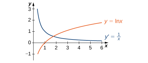
The graph of $y = ln x$ and its derivative $\frac{d y}{d x} = \frac{1}{x}$ are shown in Figure 3.35.

Graph of the function ln x along with its derivative 1/x. The function ln x is increasing on (0, + ∞). Its derivative is decreasing but greater than 0 on (0, + ∞). — Figure 3.35 $The function y = ln x$ is increasing on $(0, + \infty) .$ Its derivative $y' = \frac{1}{x}$ is greater than zero on $(0, + \infty) .$

Taking a Derivative of a Natural Logarithm

Find the derivative of $f (x) = ln (x^{3} + 3 x - 4) .$

Use Equation 3.31 directly.

\begin{matrix} f^{'} (x) & = \frac{1}{x^{3} + 3 x - 4} \cdot (3 x^{2} + 3) & Use g (x) = x^{3} + 3 x - 4 in h^{'} (x) = \frac{1}{g (x)} g^{'} (x) . \\ = \frac{3 x^{2} + 3}{x^{3} + 3 x - 4} & Rewrite. \end{matrix}

Using Properties of Logarithms in a Derivative

Find the derivative of $f (x) = ln (\frac{x^{2} sin x}{2 x + 1}) .$

At first glance, taking this derivative appears rather complicated. However, by using the properties of logarithms prior to finding the derivative, we can make the problem much simpler.

\begin{matrix} f (x) & = & ln (\frac{x^{2} sin x}{2 x + 1}) = 2 ln x + ln (sin x) - ln (2 x + 1) & Apply properties of logarithms. \\ f^{'} (x) & = & \frac{2}{x} + cot x - \frac{2}{2 x + 1} & Apply sum rule and h^{'} (x) = \frac{1}{g (x)} g^{'} (x) . \end{matrix}

Differentiate: $f (x) = ln {(3 x + 2)}^{5} .$

$f^{'} (x) = \frac{15}{3 x + 2}$

Hint

Use a property of logarithms to simplify before taking the derivative.

Now that we can differentiate the natural logarithmic function, we can use this result to find the derivatives of $y = l o g_{b} x$ and $y = b^{x}$ for $b > 0, b \neq 1 .$

Derivatives of General Exponential and Logarithmic Functions

Let $b > 0, b \neq 1,$ and let $g (x)$ be a differentiable function.

If, $y = {log}_{b} x,$ then

$\frac{d y}{d x} = \frac{1}{x ln b} .$ 3.32

More generally, if $h (x) = {log}_{b} (g (x)),$ then for all values of x for which $g (x) > 0,$

$h^{'} (x) = \frac{g^{'} (x)}{g (x) ln b} .$ 3.33
If $y = b^{x},$ then

$\frac{d y}{d x} = b^{x} ln b .$ 3.34

More generally, if $h (x) = b^{g (x)},$ then

$h^{'} (x) = b^{g (x)} g ′ (x) ln b .$ 3.35

Proof

If $y = {log}_{b} x,$ then $b^{y} = x .$ It follows that $ln (b^{y}) = ln x .$ Thus $y ln b = ln x .$ Solving for $y,$ we have $y = \frac{ln x}{ln b} .$ Differentiating and keeping in mind that $ln b$ is a constant, we see that

\frac{d y}{d x} = \frac{1}{x ln b} .

The derivative in Equation 3.32 now follows from the chain rule.

If $y = b^{x},$ then $ln y = x ln b .$ Using implicit differentiation, again keeping in mind that $ln b$ is constant, it follows that $\frac{1}{y} \frac{d y}{d x} = ln b .$ Solving for $\frac{d y}{d x}$ and substituting $y = b^{x},$ we see that

\frac{d y}{d x} = y ln b = b^{x} ln b .

The more general derivative (Equation 3.35) follows from the chain rule.

□

Applying Derivative Formulas

Find the derivative of $h (x) = \frac{3^{x}}{3^{x} + 2} .$

Use the quotient rule and Proof.

\begin{matrix} h^{'} (x) & = \frac{3^{x} ln 3 (3^{x} + 2) - 3^{x} ln 3 (3^{x})}{{(3^{x} + 2)}^{2}} & Apply the quotient rule. \\ = \frac{2 \cdot 3^{x} ln 3}{{(3^{x} + 2)}^{2}} & Simplify. \end{matrix}

Finding the Slope of a Tangent Line

Find the slope of the line tangent to the graph of $y = {log}_{2} (3 x + 1)$ at $x = 1 .$

To find the slope, we must evaluate $\frac{d y}{d x}$ at $x = 1 .$ Using Equation 3.33, we see that

\frac{d y}{d x} = \frac{3}{(3 x + 1) ln 2} .

By evaluating the derivative at $x = 1,$ we see that the tangent line has slope

\frac{d y}{d x} | \begin{array}{l} _{x = 1} \end{array} = \frac{3}{4 ln 2} = \frac{3}{ln 16} .

Find the slope for the line tangent to $y = 3^{x}$ at $x = 2 .$

$9 ln (3)$

Hint

Evaluate the derivative at $x = 2 .$

Logarithmic Differentiation

At this point, we can take derivatives of functions of the form $y = {(g (x))}^{n}$ for certain values of $n,$ as well as functions of the form $y = b^{g (x)},$ where $b > 0$ and $b \neq 1 .$ Unfortunately, we still do not know the derivatives of functions such as $y = x^{x}$ or $y = x^{π} .$ These functions require a technique called logarithmic differentiation, which allows us to differentiate any function of the form $h (x) = g {(x)}^{f (x)} .$ It can also be used to convert a very complex differentiation problem into a simpler one, such as finding the derivative of $y = \frac{x \sqrt{2 x + 1}}{e^{x} {sin}^{3} x} .$ We outline this technique in the following problem-solving strategy.

Using Logarithmic Differentiation

To differentiate $y = h (x)$ using logarithmic differentiation, take the natural logarithm of both sides of the equation to obtain $ln y = ln (h (x)) .$
Use properties of logarithms to expand $ln (h (x))$ as much as possible.
Differentiate both sides of the equation. On the left we will have $\frac{1}{y} \frac{d y}{d x} .$
Multiply both sides of the equation by $y$ to solve for $\frac{d y}{d x} .$
Replace $y$ by $h (x) .$

Using Logarithmic Differentiation

Find the derivative of $y = {(2 x^{4} + 1)}^{tan x} .$

Use logarithmic differentiation to find this derivative.

\begin{matrix} ln y & = & ln {(2 x^{4} + 1)}^{tan x} & Step 1. Take the natural logarithm of both sides. \\ ln y & = & tan x ln (2 x^{4} + 1) & Step 2. Expand using properties of logarithms. \\ \frac{1}{y} \frac{d y}{d x} & = & {sec}^{2} x ln (2 x^{4} + 1) + \frac{8 x^{3}}{2 x^{4} + 1} \cdot tan x & \begin{matrix} Step 3. Differentiate both sides. Use the \\ product rule on the right. \end{matrix} \\ \frac{d y}{d x} & = & y \cdot ({sec}^{2} x ln (2 x^{4} + 1) + \frac{8 x^{3}}{2 x^{4} + 1} \cdot tan x) & Step 4. Multiply by y on both sides. \\ \frac{d y}{d x} & = & {(2 x^{4} + 1)}^{tan x} ({sec}^{2} x ln (2 x^{4} + 1) + \frac{8 x^{3}}{2 x^{4} + 1} \cdot tan x) & Step 5. Substitute y = {(2 x^{4} + 1)}^{tan x} . \end{matrix}

Using Logarithmic Differentiation

Find the derivative of $y = \frac{x \sqrt{2 x + 1}}{e^{x} {sin}^{3} x} .$

This problem really makes use of the properties of logarithms and the differentiation rules given in this chapter.

\begin{matrix} ln y & = & ln \frac{x \sqrt{2 x + 1}}{e^{x} {sin}^{3} x} & Step 1. Take the natural logarithm of both sides. \\ ln y & = & ln x + \frac{1}{2} ln (2 x + 1) - x ln e - 3 ln sin x & Step 2. Expand using properties of logarithms. \\ \frac{1}{y} \frac{d y}{d x} & = & \frac{1}{x} + \frac{1}{2 x + 1} - 1 - 3 \frac{cos x}{sin x} & Step 3. Differentiate both sides. \\ \frac{d y}{d x} & = & y (\frac{1}{x} + \frac{1}{2 x + 1} - 1 - 3 cot x) & Step 4. Multiply by y on both sides. \\ \frac{d y}{d x} & = & \frac{x \sqrt{2 x + 1}}{e^{x} {sin}^{3} x} (\frac{1}{x} + \frac{1}{2 x + 1} - 1 - 3 cot x) & Step 5. Substitute y = \frac{x \sqrt{2 x + 1}}{e^{x} {sin}^{3} x} . \end{matrix}

Extending the Power Rule

Find the derivative of $y = x^{r}$ where $r$ is an arbitrary real number.

The process is the same as in Example 3.82, though with fewer complications.

\begin{matrix} ln y & = & ln x^{r} & Step 1. Take the natural logarithm of both sides. \\ ln y & = & r ln x & Step 2. Expand using properties of logarithms. \\ \frac{1}{y} \frac{d y}{d x} & = & r \frac{1}{x} & Step 3. Differentiate both sides. \\ \frac{d y}{d x} & = & y \frac{r}{x} & Step 4. Multiply by y on both sides. \\ \frac{d y}{d x} & = & x^{r} \frac{r}{x} & Step 5. Substitute y = x^{r} . \\ \frac{d y}{d x} & = & r x^{r - 1} & Simplify. \end{matrix}

Use logarithmic differentiation to find the derivative of $y = x^{x} .$

$\frac{d y}{d x} = x^{x} (1 + ln x)$

Hint

Follow the problem solving strategy.

Find the derivative of $y = {(tan x)}^{π} .$

$y^{'} = π {(tan x)}^{π - 1} {sec}^{2} x$

Hint

Use the result from Example 3.83.

Key Concepts

On the basis of the assumption that the exponential function $y = b^{x}, b > 0$ is continuous everywhere and differentiable at 0, this function is differentiable everywhere and there is a formula for its derivative.
We can use a formula to find the derivative of $y = ln x,$ and the relationship ${log}_{b} x = \frac{ln x}{ln b}$ allows us to extend our differentiation formulas to include logarithms with arbitrary bases.
Logarithmic differentiation allows us to differentiate functions of the form $y = g {(x)}^{f (x)}$ or very complex functions by taking the natural logarithm of both sides and exploiting the properties of logarithms before differentiating.

Key Equations

Derivative of the natural exponential function	$\frac{d}{d x} (e^{g (x)}) = e^{g (x)} g^{'} (x)$
Derivative of the natural logarithmic function	$\frac{d}{d x} (ln g (x)) = \frac{1}{g (x)} g^{'} (x)$
Derivative of the general exponential function	$\frac{d}{d x} (b^{g (x)}) = b^{g (x)} g^{'} (x) ln b$
Derivative of the general logarithmic function	$\frac{d}{d x} ({log}_{b} g (x)) = \frac{g^{'} (x)}{g (x) ln b}$

For the following exercises, find $f^{'} (x)$ for each function.

$f (x) = x^{2} e^{x}$

$2 x e^{x} + x^{2} e^{x}$

$f (x) = \frac{e^{− x}}{x}$

$f (x) = e^{x^{3} ln x}$

$e^{x^{3} ln x} (3 x^{2} ln x + x^{2})$

$f (x) = \sqrt{e^{2 x} + 2 x}$

$f (x) = \frac{e^{x} - e^{− x}}{e^{x} + e^{− x}}$

$\frac{4}{{(e^{x} + e^{− x})}^{2}}$

$f (x) = \frac{10^{x}}{ln 10}$

$f (x) = 2^{4 x} + 4 x^{2}$

$2^{4 x + 2} \cdot ln 2 + 8 x$

$f (x) = 3^{sin 3 x}$

$f (x) = x^{π} \cdot π^{x}$

$π x^{π - 1} \cdot π^{x} + x^{π} \cdot π^{x} ln π$

$f (x) = ln (4 x^{3} + x)$

$f (x) = ln \sqrt{5 x - 7}$

$\frac{5}{2 (5 x - 7)}$

$f (x) = x^{2} ln 9 x$

$f (x) = log (sec x)$

$\frac{tan x}{ln 10}$

$f (x) = {log}_{7} {(6 x^{4} + 3)}^{5}$

$f (x) = 2^{x} \cdot {log}_{3} 7^{x^{2} - 4}$

$2^{x} \cdot ln 2 \cdot {log}_{3} 7^{x^{2} - 4} + 2^{x} \cdot \frac{2 x ln 7}{ln 3}$

For the following exercises, use logarithmic differentiation to find $\frac{d y}{d x} .$

$y = x^{\sqrt{x}}$

$y = {(sin 2 x)}^{4 x}$

${(sin 2 x)}^{4 x} [4 \cdot ln (sin 2 x) + 8 x \cdot cot 2 x]$

$y = {(ln x)}^{ln x}$

$y = x^{{log}_{2} x}$

$x^{{log}_{2} x} \cdot \frac{2 ln x}{x ln 2}$

$y = {(x^{2} - 1)}^{ln x}$

$y = x^{cot x}$

$x^{cot x} \cdot [− {csc}^{2} x \cdot ln x + \frac{cot x}{x}]$

$y = \frac{x + 11}{\sqrt[3]{x^{2} - 4}}$

$y = x^{−1 / 2} {(x^{2} + 3)}^{2 / 3} {(3 x - 4)}^{4}$

$x^{−1 / 2} {(x^{2} + 3)}^{2 / 3} {(3 x - 4)}^{4} \cdot [\frac{−1}{2 x} + \frac{4 x}{3 (x^{2} + 3)} + \frac{12}{3 x - 4}]$

[T] Find an equation of the tangent line to the graph of $f (x) = 4 x e^{(x^{2} - 1)}$ at the point where

$x = −1 .$ Graph both the function and the tangent line.

[T] Find an equation of the line that is normal to the graph of $f (x) = x \cdot 5^{x}$ at the point where $x = 1 .$ Graph both the function and the normal line.

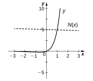
The function starts at (−3, 0), decreases slightly and then increases through the origin and increases to (1.25, 10). There is a straight line marked T(x) with slope −1/(5 + 5 ln 5) and y intercept 5 + 1/(5 + 5 ln 5).

$y = \frac{−1}{5 + 5 ln 5} x + (5 + \frac{1}{5 + 5 ln 5})$

[T] Find an equation of the tangent line to the graph of $x^{3} - x ln y + y^{3} = 2 x + 5$ at the point (2, 1). (Hint: Use implicit differentiation to find $\frac{d y}{d x} .)$ Graph both the curve and the tangent line.

Consider the function $y = x^{1 / x}$ for $x > 0 .$

Determine the points on the graph where the tangent line is horizontal.
Determine the points on the graph where $y^{'} > 0$ and those where $y^{'} < 0 .$

a. $x = e ~ 2.718$ b. $y' > 0 on (0, e); y' < 0 on (e, \infty)$

The formula $I (t) = \frac{sin t}{e^{t}}$ is the formula for a decaying alternating current.

Complete the following table with the appropriate values.

$t$ $\frac{sin t}{e^{t}}$
0 (i)
$\frac{π}{2}$ (ii)
$π$ (iii)
$\frac{3 π}{2}$ (iv)
$2 π$ (v)
$\frac{5 π}{2}$ (vi)
$3 π$ (vii)
$\frac{7 π}{2}$ (viii)
$4 π$ (ix)
This table has two columns and 10 rows. The first column reads t, 0, π/2, π, 3π/2, 2π, 5π/2, 3π, 7π/2, and 4π. The second column reads (sin t)/et, (i), (ii), (iii), (iv), (v), (vi), (vii), (viii), and (ix).
Using only the values in the table, determine where the tangent line to the graph of $I (t)$ is horizontal.

$t$	$\frac{sin t}{e^{t}}$
0	(i)
$\frac{π}{2}$	(ii)
$π$	(iii)
$\frac{3 π}{2}$	(iv)
$2 π$	(v)
$\frac{5 π}{2}$	(vi)
$3 π$	(vii)
$\frac{7 π}{2}$	(viii)
$4 π$	(ix)

[T] The population of Toledo, Ohio, in 2000 was approximately 500,000. Assume the population is increasing at a rate of 5% per year.

Write the exponential function that relates the total population as a function of $t .$
Use a. to determine the rate at which the population is increasing in $t$ years.
Use b. to determine the rate at which the population is increasing in 10 years.

a. $P = 500,000 {(1.05)}^{t}$ individuals b. $P^{'} (t) = 24395 \cdot {(1.05)}^{t}$ individuals per year c. $39,737$ individuals per year

[T] An isotope of the element erbium has a half-life of approximately 12 hours. Initially there are 9 grams of the isotope present.

Write the exponential function that relates the amount of substance remaining as a function of $t,$ measured in hours.
Use a. to determine the rate at which the substance is decaying in $t$ hours.
Use b. to determine the rate of decay at $t = 4$ hours.

[T] The number of cases of influenza in New York City from the beginning of 1960 to the beginning of 1964 is modeled by the function

$N (t) = 5.3 e^{0.093 t^{2} - 0.87 t}, (0 \leq t \leq 4),$ where $N (t)$ gives the number of cases (in thousands) and t is measured in years, with $t = 0$ corresponding to the beginning of 1960.

Show work that evaluates $N (0)$ and $N (4) .$ Briefly describe what these values indicate about the disease in New York City.
Show work that evaluates $N^{'} (0)$ and $N^{'} (3) .$ Briefly describe what these values indicate about the disease in New York City.

a. At the beginning of 1960 there were 5.3 thousand cases of the disease in New York City. At the beginning of 1964 there were approximately 723 cases of the disease in the United States. b. At the beginning of 1960 the number of cases of the disease was decreasing at rate of $−4.611$ thousand per year; at the beginning of 1963, the number of cases of the disease was decreasing at a rate of $−0.2808$ thousand per year.

[T] The relative rate of change of a differentiable function $y = f (x)$ is given by $\frac{100 \cdot f^{'} (x)}{f (x)} % .$ One model for population growth is a Gompertz growth function, given by $P (x) = a e^{− b \cdot e^{− c x}}$ where $a, b,$ and $c$ are constants.

Find the relative rate of change formula for the generic Gompertz function.
Use a. to find the relative rate of change of a population in $x = 20$ months when $a = 204, b = 0.0198,$ and $c = 0.15 .$
Briefly interpret what the result of b. means.

For the following exercises, use the population of New York City from 1790 to 1860, given in the following table.

Table 3.8 New York City Population Over Time Source: http://en.wikipedia.org/wiki/Largest_cities_in_the_United_States
_by_population_by_decade.
Years since 1790	Population
0	33,131
10	60,515
20	96,373
30	123,706
40	202,300
50	312,710
60	515,547
70	813,669

[T] Using a computer program or a calculator, fit a growth curve to the data of the form $p = a b^{t} .$

$p = 35741 {(1.045)}^{t}$

[T] Using the exponential best fit for the data, write a table containing the derivatives evaluated at each year.

[T] Using the exponential best fit for the data, write a table containing the second derivatives evaluated at each year.

Years since 1790	$P^{″}$
0	69.25
10	107.5
20	167.0
30	259.4
40	402.8
50	625.5
60	971.4
70	1508.5

[T] Using the tables of first and second derivatives and the best fit, answer the following questions:

Will the model be accurate in predicting the future population of New York City? Why or why not?
Estimate the population in 2010. Was the prediction correct from a.?

Chapter Review Exercises

True or False? Justify the answer with a proof or a counterexample.

Every function has a derivative.

False.

A continuous function has a continuous derivative.

A continuous function has a derivative.

False

If a function is differentiable, it is continuous.

Use the limit definition of the derivative to exactly evaluate the derivative.

$f (x) = \sqrt{x + 4}$

$\frac{1}{2 \sqrt{x + 4}}$

$f (x) = \frac{3}{x}$

Find the derivatives of the following functions.

$f (x) = 3 x^{3} - \frac{4}{x^{2}}$

$9 x^{2} + \frac{8}{x^{3}}$

$f (x) = {(4 - x^{2})}^{3}$

$f (x) = e^{sin x}$

$e^{sin x} cos x$

$f (x) = ln (x + 2)$

$f (x) = x^{2} cos x + x tan (x)$

$x {sec}^{2} (x) + 2 x cos (x) + tan (x) - x^{2} sin (x)$

$f (x) = \sqrt{3 x^{2} + 2}$

$f (x) = \frac{x}{4} {sin}^{−1} (x)$

$\frac{1}{4} (\frac{x}{\sqrt{1 - x^{2}}} + {sin}^{−1} (x))$

$x^{2} y = (y + 2) + x y sin (x)$

Find the following derivatives of various orders.

First derivative of $y = x ln (x) cos x$

$cos x \cdot (ln x + 1) - x ln (x) sin x$

Third derivative of $y = {(3 x + 2)}^{2}$

Second derivative of $y = 4^{x} + x^{2} sin (x)$

$4^{x} {(ln 4)}^{2} + 2 sin x + 4 x cos x - x^{2} sin x$

Find an equation of the tangent line to the following equations at the specified point.

$y = {cos}^{−1} (x) + x$ at $x = 0$

$y = x + e^{x} - \frac{1}{x}$ at $x = 1$

$T = (2 + e) x - 2$

Draw the derivative for the following graphs.

The function begins at (−3, 0.5) and decreases to a local minimum at (−2.3, −2). Then the function increases through (−1.5, 0) and slows its increase through (0, 2). It then slowly increases to a local maximum at (2.3, 6) before decreasing to (3, 3).

The function decreases linearly from (−1, 4) to the origin, at which point it increases as x2, passing through (1, 1) and (2, 4).

The function is the straight line y = −4 until x = 0, at which point it becomes a straight line starting at the origin with slope 2. There is no value assigned for this function at x = 0.

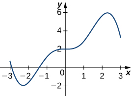
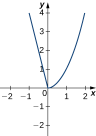
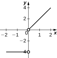
The following questions concern the water level in Ocean City, New Jersey, in January, which can be approximated by $w (t) = 1.9 + 2.9 cos (\frac{π}{6} t),$ where t is measured in hours after midnight, and the height is measured in feet.

Find and graph the derivative. What is the physical meaning?

Find $w^{'} (3) .$ What is the physical meaning of this value?

$w^{'} (3) = - \frac{2.9 π}{6} .$ At 3 a.m. the tide is decreasing at a rate of 1.518 ft/hr.

The following questions consider the wind speeds of Hurricane Katrina, which affected New Orleans, Louisiana, in August 2005. The data are displayed in a table.

Table 3.9 Wind Speeds of Hurricane Katrina Source: http://news.nationalgeographic.com/news/2005/09/0914_050914_katrina_timeline.html.
Hours after Midnight, August 26	Wind Speed (mph)
1	45
5	75
11	100
29	115
49	145
58	175
73	155
81	125
85	95
107	35

Using the table, estimate the derivative of the wind speed at hour 39. What is the physical meaning?

Estimate the derivative of the wind speed at hour 83. What is the physical meaning?

$−7.5 .$ The wind speed is decreasing at a rate of 7.5 mph/hr

Glossary

logarithmic differentiation: is a technique that allows us to differentiate a function by first taking the natural logarithm of both sides of an equation, applying properties of logarithms to simplify the equation, and differentiating implicitly