- Describe the epsilon-delta definition of a limit.
- Apply the epsilon-delta definition to find the limit of a function.
- Describe the epsilon-delta definitions of one-sided limits and infinite limits.
- Use the epsilon-delta definition to prove the limit laws.
By now you have progressed from the very informal definition of a limit in the introduction of this chapter to the intuitive understanding of a limit. At this point, you should have a very strong intuitive sense of what the limit of a function means and how you can find it. In this section, we convert this intuitive idea of a limit into a formal definition using precise mathematical language. The formal definition of a limit is quite possibly one of the most challenging definitions you will encounter early in your study of calculus; however, it is well worth any effort you make to reconcile it with your intuitive notion of a limit. Understanding this definition is the key that opens the door to a better understanding of calculus.
Quantifying Closeness
Before stating the formal definition of a limit, we must introduce a few preliminary ideas. Recall that the distance between two points a and b on a number line is given by
- The statement may be interpreted as: The distance between and L is less than ε.
- The statement may be interpreted as: and the distance between x and a is less than δ.
It is also important to look at the following equivalences for absolute value:
- The statement is equivalent to the statement
- The statement is equivalent to the statement and
With these clarifications, we can state the formal epsilon-delta definition of the limit.
Let be defined for all over an open interval containing a. Let L be a real number. Then
if, for every there exists a such that if then
This definition may seem rather complex from a mathematical point of view, but it becomes easier to understand if we break it down phrase by phrase. The statement itself involves something called a universal quantifier (for every an existential quantifier (there exists a and, last, a conditional statement (if then Let’s take a look at Table 2.9, which breaks down the definition and translates each part.
| Definition | Translation |
|---|---|
| 1. For every | 1. For every positive distance ε from L, |
| 2. there exists a | 2. There is a positive distance from a, |
| 3. such that | 3. such that |
| 4. if then | 4. if x is closer than to a and then is closer than ε to L. |
A table with two columns and five rows. The first row has the headers “definition” and “translation,” from mathematical symbols to words. The second row has defines “for every epsilon less than 0” as “for every positive distance epsilon from L,” the third row defines “there exists a delta less than 0” as “there is a positive difference delta from a,” and the fourth row defines “if 0 is less than the absolute value of x –a, and that is less than delta, then the absolute value of the function of x minus L is less than epsilon” as “if x is closer than delta to a and x is not equal to a, then the function of x is closer than epsilon to L.”
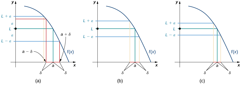
We can get a better handle on this definition by looking at the definition geometrically. Figure 2.39 shows possible values of for various choices of for a given function a number a, and a limit L at a. Notice that as we choose smaller values of ε (the distance between the function and the limit), we can always find a small enough so that if we have chosen an x value within of a, then the value of is within ε of the limit L.
Visit the following applet to experiment with finding values of for selected values of ε:
Example 2.39 shows how you can use this definition to prove a statement about the limit of a specific function at a specified value.
Prove that
Let
The first part of the definition begins “For every This means we must prove that whatever follows is true no matter what positive value of ε is chosen. By stating “Let we signal our intent to do so.
Choose
The definition continues with “there exists a ” The phrase “there exists” in a mathematical statement is always a signal for a scavenger hunt. In other words, we must go and find So, where exactly did come from? There are two basic approaches to tracking down One method is purely algebraic and the other is geometric.
We begin by tackling the problem from an algebraic point of view. Since ultimately we want we begin by manipulating this expression: is equivalent to which in turn is equivalent to Last, this is equivalent to Thus, it would seem that is appropriate.
We may also find through geometric methods. Figure 2.40 demonstrates how this is done.
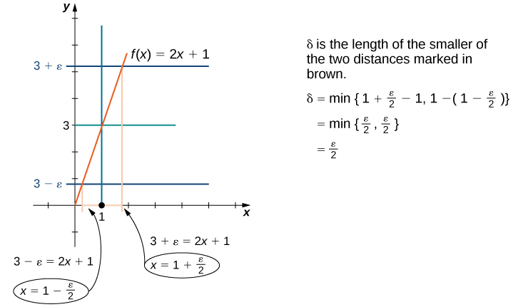
Assume When has been chosen, our goal is to show that if then To prove any statement of the form “If this, then that,” we begin by assuming “this” and trying to get “that.”
Thus,
The following Problem-Solving Strategy summarizes the type of proof we worked out in Example 2.39.
- Let’s begin the proof with the following statement: Let
- Next, we need to obtain a value for After we have obtained this value, we make the following statement, filling in the blank with our choice of : Choose
- The next statement in the proof should be (at this point, we fill in our given value for a):
Assume - Next, based on this assumption, we need to show that where and L are our function and our limit L. At some point, we need to use
- We conclude our proof with the statement: Therefore,
Complete the proof that by filling in the blanks.
Let _____.
Choose
Assume
Thus,
We begin by filling in the blanks where the choices are specified by the definition. Thus, we have
Let
Choose
Assume (or equivalently,
Thus,
Focusing on the final line of the proof, we see that we should choose
We now complete the final write-up of the proof:
Let
Choose
Assume (or equivalently,
Thus,
Complete the proof that by filling in the blanks.
Let _______.
Choose
Assume
Thus,
Therefore,
Let choose assume
Thus,
Therefore,
Follow the outline in the Problem-Solving Strategy that we worked out in full in Example 2.40.
In Example 2.39 and Example 2.40, the proofs were fairly straightforward, since the functions with which we were working were linear. In Example 2.41, we see how to modify the proof to accommodate a nonlinear function.
Prove that
- Let The first part of the definition begins “For every so we must prove that whatever follows is true no matter what positive value of ε is chosen. By stating “Let we signal our intent to do so.
- Without loss of generality, assume Two questions present themselves: Why do we want and why is it okay to make this assumption? In answer to the first question: Later on, in the process of solving for we will discover that involves the quantity Consequently, we need In answer to the second question: If we can find that “works” for then it will “work” for any as well. Keep in mind that, although it is always okay to put an upper bound on ε, it is never okay to put a lower bound (other than zero) on ε.
- Choose Figure 2.41 shows how we made this choice of
![This graph shows how to find delta geometrically for a given epsilon for the above proof. First, the function f(x) = x^2 is drawn from [-1, 3]. On the y axis, the proposed limit 4 is marked, and the line y=4 is drawn to intersect with the function at (2,4). For a given epsilon, point 4 + epsilon and 4 – epsilon are marked on the y axis above and below 4. Blue lines are drawn from these points to intersect with the function, where pink lines are drawn from the point of intersection to the x axis. These lines land on either side of x=2. Next, we solve for these x values, which have to be positive here. The first is x^2 = 4 – epsilon, which simplifies to x = sqrt(4-epsilon). The next is x^2 = 4 + epsilon, which simplifies to x = sqrt(4 + epsilon). Delta is the smaller of the two distances, so it is the min of (2 – sqrt(4 – epsilon) and sqrt(4 + epsilon) – 2).](/calculus-bundle/media/CNX_Calc_Figure_02_05_003.jpg)
Figure 2.41 This graph shows how we find δ geometrically for a given ε for the proof in Example 2.41. - We must show: If then so we must begin by assuming
We don’t really need (in other words, for this proof. Since it is okay to drop
Hence,
Recall that Thus, and consequently We also use here. We might ask at this point: Why did we substitute for on the left-hand side of the inequality and on the right-hand side of the inequality? If we look at Figure 2.41, we see that corresponds to the distance on the left of 2 on the x-axis and corresponds to the distance on the right. Thus,
We simplify the expression on the left:
Then, we add 2 to all parts of the inequality:
We square all parts of the inequality. It is okay to do so, since all parts of the inequality are positive:
We subtract 4 from all parts of the inequality:
Last,
- Therefore,
Find δ corresponding to for a proof that
Choose
Draw a graph similar to the one in Example 2.41.
The geometric approach to proving that the limit of a function takes on a specific value works quite well for some functions. Also, the insight into the formal definition of the limit that this method provides is invaluable. However, we may also approach limit proofs from a purely algebraic point of view. In many cases, an algebraic approach may not only provide us with additional insight into the definition, it may prove to be simpler as well. Furthermore, an algebraic approach is the primary tool used in proofs of statements about limits. For Example 2.42, we take on a purely algebraic approach.
Prove that
Let’s use our outline from the Problem-Solving Strategy:
- Let
- Choose This choice of may appear odd at first glance, but it was obtained by taking a look at our ultimate desired inequality: This inequality is equivalent to At this point, the temptation simply to choose is very strong. Unfortunately, our choice of must depend on ε only and no other variable. If we can replace by a numerical value, our problem can be resolved. This is the place where assuming comes into play. The choice of here is arbitrary. We could have just as easily used any other positive number. In some proofs, greater care in this choice may be necessary. Now, since and we are able to show that Consequently, At this point we realize that we also need Thus, we choose
- Assume Thus,
Since we may conclude that Thus, by subtracting 4 from all parts of the inequality, we obtain Consequently, This gives us
Therefore,
Complete the proof that
Let choose assume
Since we may conclude that Thus, Hence,
Use Example 2.42 as a guide.
You will find that, in general, the more complex a function, the more likely it is that the algebraic approach is the easiest to apply. The algebraic approach is also more useful in proving statements about limits.
Proving Limit Laws
We now demonstrate how to use the epsilon-delta definition of a limit to construct a rigorous proof of one of the limit laws. The triangle inequality is used at a key point of the proof, so we first review this key property of absolute value.
The triangle inequality states that if a and b are any real numbers, then
Proof
We prove the following limit law: If and then
Let
Choose so that if then
Choose so that if then
Choose
Assume
Thus,
Hence,
□
We now explore what it means for a limit not to exist. The limit does not exist if there is no real number L for which Thus, for all real numbers L, To understand what this means, we look at each part of the definition of together with its opposite. A translation of the definition is given in Table 2.10.
| Definition | Opposite |
|---|---|
| 1. For every | 1. There exists so that |
| 2. there exists a so that | 2. for every |
| 3. if then | 3. There is an x satisfying so that |
A table with two columns and four rows. The top row contains the headers “definition” and “opposite.” The second row contains the definition “for every epsilon < 0” and the opposite “there exists an epsilon greater than zero so that.” The third row contains the definition “there exists a delta greater than 0, so that” and the opposite “for every delta greater than 0.” The last row contains the definition “if 0 is less than the absolute value of x-a, which is less than delta, then the absolute value of f(x) – L is less than epsilon” and the opposite “there is an x satisfying 0 is less than the absolute value of x – a, which is less than delta, so that the absolute value of f() – L is greater than or equal to epsilon.
Finally, we may state what it means for a limit not to exist. The limit does not exist if for every real number L, there exists a real number so that for all there is an x satisfying so that Let’s apply this in Example 2.43 to show that a limit does not exist.
Show that does not exist. The graph of is shown here:
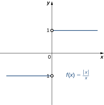
Suppose that L is a candidate for a limit. Choose
Let Either or If then let Thus,
and
On the other hand, if then let Thus,
and
Thus, for any value of L,
One-Sided and Infinite Limits
Just as we first gained an intuitive understanding of limits and then moved on to a more rigorous definition of a limit, we now revisit one-sided limits. To do this, we modify the epsilon-delta definition of a limit to give formal epsilon-delta definitions for limits from the right and left at a point. These definitions only require slight modifications from the definition of the limit. In the definition of the limit from the right, the inequality replaces which ensures that we only consider values of x that are greater than (to the right of) a. Similarly, in the definition of the limit from the left, the inequality replaces which ensures that we only consider values of x that are less than (to the left of) a.
Limit from the Right: Let be defined over an open interval of the form where Then,
if for every there exists a such that if then
Limit from the Left: Let be defined over an open interval of the form where Then,
if for every there exists a such that if then
Prove that
Let
Choose Since we ultimately want we manipulate this inequality to get or, equivalently, making a clear choice. We may also determine geometrically, as shown in Figure 2.42.
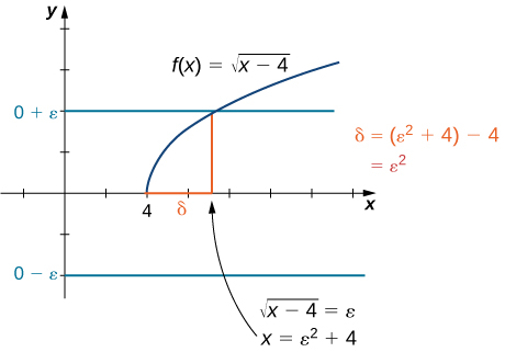
Assume Thus, Hence, Finally,
Therefore,
Find corresponding to ε for a proof that
Sketch the graph and use Example 2.44 as a solving guide.
We conclude the process of converting our intuitive ideas of various types of limits to rigorous formal definitions by pursuing a formal definition of infinite limits. To have we want the values of the function to get larger and larger as x approaches a. Instead of the requirement that for arbitrarily small ε when for small enough we want for arbitrarily large positive M when for small enough Figure 2.43 illustrates this idea by showing the value of for successively larger values of M.
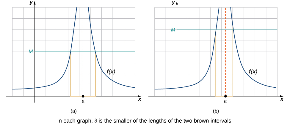
Let be defined for all in an open interval containing a. Then, we have an infinite limit
if for every there exists such that if then
Let be defined for all in an open interval containing a. Then, we have a negative infinite limit
if for every there exists such that if then
Key Concepts
- The intuitive notion of a limit may be converted into a rigorous mathematical definition known as the epsilon-delta definition of the limit.
- The epsilon-delta definition may be used to prove statements about limits.
- The epsilon-delta definition of a limit may be modified to define one-sided limits.
In the following exercises, write the appropriate - definition for each of the given statements.
For every there exists a so that if then
For every there exists a so that if then
The following graph of the function f satisfies In the following exercises, determine a value of that satisfies each statement.
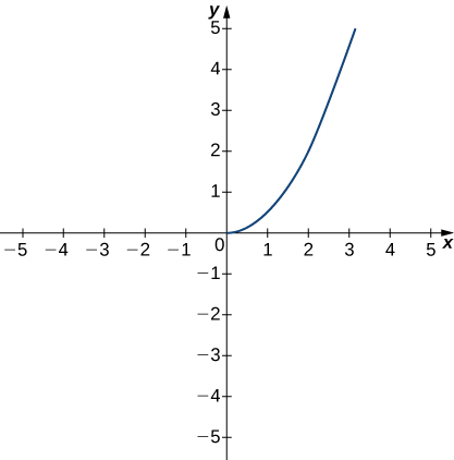
If then
If then
The following graph of the function f satisfies In the following exercises, determine a value of that satisfies each statement.
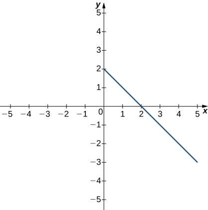
If then
If then
The following graph of the function f satisfies In the following exercises, for each value of ε, find a value of such that the precise definition of limit holds true.
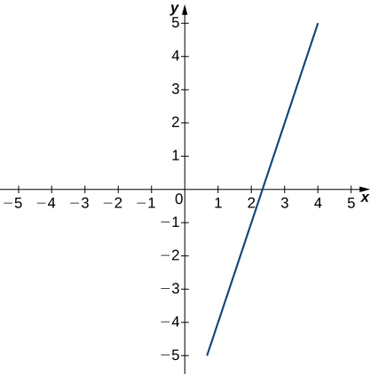
[T] In the following exercises, use a graphing calculator to find a number such that the statements hold true.
whenever
In the following exercises, use the precise definition of limit to prove the given limits.
Let If then
Let If then
In the following exercises, use the precise definition of limit to prove the given one-sided limits.
Let If then
Let If then
In the following exercises, use the precise definition of limit to prove the given infinite limits.
Let If then
An engineer is using a machine to cut a flat square of Aerogel of area 144 cm2. If there is a maximum error tolerance in the area of 8 cm2, how accurately must the engineer cut on the side, assuming all sides have the same length? How do these numbers relate to ε, a, and L?
The engineer must cut within 0.328 cm of 12 cm on each side;
Use the precise definition of limit to prove that the following limit does not exist:
Using precise definitions of limits, prove that does not exist, given that is the ceiling function. (Hint: Try any
Answers may vary.
Using precise definitions of limits, prove that does not exist: (Hint: Think about how you can always choose a rational number but
Using precise definitions of limits, determine for (Hint: Break into two cases, x rational and x irrational.)
0
Using the function from the previous exercise, use the precise definition of limits to show that does not exist for
For the following exercises, suppose that and both exist. Use the precise definition of limits to prove the following limit laws:
for any real constant c (Hint: Consider two cases: and
(Hint:
Answers may vary.
Chapter Review Exercises
True or False. In the following exercises, justify your answer with a proof or a counterexample.
A function has to be continuous at if the exists.
You can use the quotient rule to evaluate
False
If there is a vertical asymptote at for the function then f is undefined at the point
If does not exist, then f is undefined at the point
False. A removable discontinuity is possible.
Using the graph, find each limit or explain why the limit does not exist.
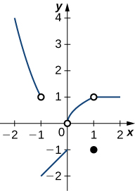
In the following exercises, evaluate the limit algebraically or explain why the limit does not exist.
5
DNE
−4;
In the following exercises, use the squeeze theorem to prove the limit.
Since then Since it follows that
Determine the domain such that the function is continuous over its domain.
In the following exercises, determine the value of c such that the function remains continuous. Draw your resulting function to ensure it is continuous.
In the following exercises, use the precise definition of limit to prove the limit.
A ball is thrown into the air and the vertical position is given by Use the Intermediate Value Theorem to show that the ball must land on the ground sometime between 5 sec and 6 sec after the throw.
A particle moving along a line has a displacement according to the function where x is measured in meters and t is measured in seconds. Find the average velocity over the time period
From the previous exercises, estimate the instantaneous velocity at by checking the average velocity within
Glossary
- epsilon-delta definition of the limit
- if for every there exists a such that if then
- triangle inequality
- If a and b are any real numbers, then
In this part of the proof, we started with and used our assumption in a key part of the chain of inequalities to get to be less than ε. We could just as easily have manipulated the assumed inequality to arrive at as follows:
Therefore, (Having completed the proof, we state what we have accomplished.)
After removing all the remarks, here is a final version of the proof:
Let
Choose
Assume
Thus,
Therefore,