7.5 Magnetic Field of an Infinitely-Long Straight Current-Bearing Wire

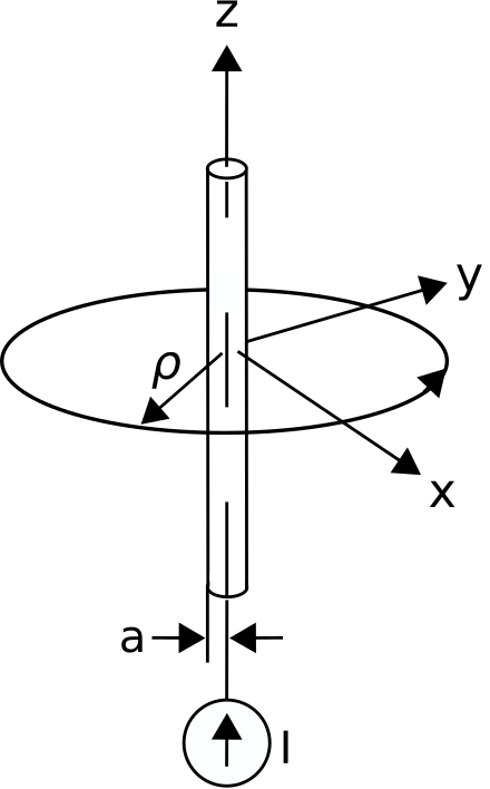
In this section, we use the magnetostatic form of Ampere’s Circuital Law (ACL) (Section 7.4) to determine the magnetic field due to a steady current \(I\) (units of A) in an infinitely-long straight wire. The problem is illustrated in Figure 7.3. The wire is an electrically-conducting circular cylinder of radius \(a\). Since the wire is a cylinder, the problem is easiest to work in cylindrical coordinates with the wire aligned along the \(z\) axis.

Here’s the relevant form of ACL:

where \(I_{encl}\) is the current enclosed by the closed path \({\mathcal C}\). ACL works for any closed path, so to exploit the symmetry of the cylindrical coordinate system we choose a circular path of radius \(\rho\) in the \(z=0\) plane, centered at the origin. With this choice we have

For \(\rho<a\), we see that \(I_{encl}<I\). a steady (DC) current will be distributed uniformly throughout the wire (Section 6.4). Since the current is uniformly distributed over the cross section, \(I_{encl}\) is less than the total current \(I\) by the same factor that the area enclosed by \({\mathcal C}\) is less than \(\pi a^2\), the cross-sectional area of the wire. The area enclosed by \({\mathcal C}\) is simply \(\pi \rho^2\), so we have

For the choice of \({\mathcal C}\) made above, Equation 7.7 becomes

Note that we have chosen to integrate in the \(+\phi\) direction. Therefore, the right-hand rule specifies that positive \(I_{encl}\) corresponds to current flowing in the \(+z\) direction, which is consistent with the direction indicated in Figure 7.3. (Here’s an excellent exercise to test your understanding. Change the direction of the path of integration and confirm that you get the same result obtained at the end of this section. Changing the direction of integration should not change the magnetic field associated with the current!)

The simplest way to solve for \({\bf H}\) from Equation 7.10 is to use a symmetry argument, which proceeds as follows:

• Since the distribution of current is uniform and infinite in the \(z\)-dimension, \({\bf H}\) can’t depend on \(z\), and so \({\bf H}\cdot\hat{\bf z}\) must be zero everywhere.

• The problem is identical after any amount of rotation in \(\phi\); therefore, the magnitude of \({\bf H}\) cannot depend on \(\phi\). This is a form of radial symmetry. Since we determined above that \({\bf H}\) can’t depend on \(z\) either, it must be that the magnitude of \({\bf H}\) can depend only on \(\rho\).

• The radial symmetry of the problem also requires that \({\bf H}\cdot\hat{\bf \rho}\) be equal to zero. If this were not the case, then the field would not be radially symmetric. Since we determined above that \({\bf H}\cdot\hat{\bf z}\) is also zero, \({\bf H}\) must be entirely \(\pm\hat{\bf \phi}\)-directed.

From the above considerations, the most general form of the magnetic field intensity can be written \({\bf H} = \hat{\bf \phi}H(\rho)\). Substituting this into Equation 7.10, we obtain

Therefore, \(H(\rho)=I_{encl}/2\pi \rho\). Reassociating the known direction, we obtain:

Therefore, the field outside of the wire is:

whereas the field inside the wire is:

(By the way, this is a good time for a units check.)

Note that as \(\rho\) increases from zero to \(a\) (i.e., inside the wire), the magnetic field is proportional to \(\rho\) and therefore increases. However, as \(\rho\) continues to increase beyond \(a\) (i.e., outside the wire), the magnetic field is proportional to \(\rho^{-1}\) and therefore decreases.

If desired, the associated magnetic flux density can be obtained using \({\bf B} = \mu {\bf H}\).

Summarizing:

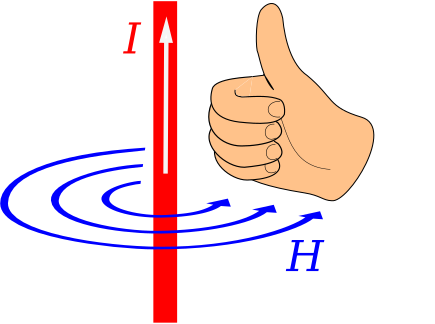
Finally, we point out another “right-hand rule” that emerges from this solution, shown in Figure 7.4 and summarized below:

This simple rule turns out to be handy in quickly determining the relationship between the directions of the magnetic field and current flow in many other problems, and so is well worth committing to memory.