In homogeneous media, electromagnetic quantities vary smoothly and continuously. At an interface between dissimilar media, however, it is possible for electromagnetic quantities to be discontinuous. These discontinuities can be described mathematically as boundary conditions and used to to constrain solutions for the associated electromagnetic quantities. In this section, we derive boundary conditions on the electric field intensity \({\bf E}\).
To begin, consider a region consisting of only two media that meet at an interface defined by the mathematical surface \({\mathcal S}\), as shown in Figure 5.7.
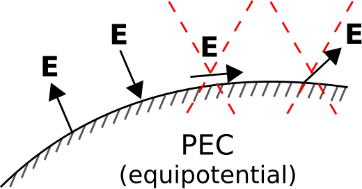
If either one of the materials is a perfect electrical conductor (PEC), then \({\mathcal S}\) is an equipotential surface; i.e., the electric potential \(V\) is constant everywhere on \({\mathcal S}\). Since \({\bf E}\) is proportional to the spatial rate of change of potential (recall \({\bf E}=-\nabla V\); Section 5.14), we find:
The component of \({\bf E}\) that is tangent to a perfectly-conducting surface is zero.
This is sometimes expressed informally as follows:
where “\(E_{tan}\)” is understood to be the component of \({\bf E}\) that is tangent to \({\mathcal S}\). Since the tangential component of \({\bf E}\) on the surface of a perfect conductor is zero, the electric field at the surface must be oriented entirely in the direction perpendicular to the surface, as shown in Figure 5.7.
The following equation expresses precisely the same idea, but includes the calculation of the tangential component as part of the statement:
where \(\hat{\bf n}\) is either normal (i.e., unit vector perpendicular to the surface) to each point on \({\mathcal S}\). This expression works because the cross product of any two vectors is perpendicular to either vector (Section 4.1), and any vector which is perpendicular to \(\hat{\bf n}\) is tangent to \({\mathcal S}\).
We now determine a more general boundary condition that applies even when neither of the media bordering \({\mathcal S}\) is a perfect conductor. The desired boundary condition can be obtained directly from Kirchoff’s Voltage Law (KVL; Section 5.10):
Let the closed path of integration take the form of a rectangle centered on \({\mathcal S}\), as shown in Figure 5.8.
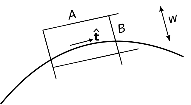
Let the sides \(A\), \(B\), \(C\), and \(D\) be perpendicular or parallel to the surface, respectively. Let the length of the perpendicular sides be \(w\), and let the length of the parallel sides be \(l\). From KVL we have
Now, let us reduce \(w\) and \(l\) together while (1) maintaining a constant ratio \(w/l\ll 1\) and (2) keeping \(\mathcal{C}\) centered on \(\mathcal{S}\). In this process, the contributions from the \(B\) and \(D\) segments become equal in magnitude but opposite in sign; i.e.,
This leaves
Let us define the unit vector \(\hat{\bf t}\) (“tangent”) as shown in Figure 5.8. When the lengths of sides \(A\) and \(C\) become sufficiently small, we can write the above expression as follows:
where \({\bf E}_1\) and \({\bf E}_2\) are the fields evaluated on the two sides of the boundary and \(\Delta l\to 0\) is the length of sides \(A\) and \(C\) while this is happening. Note that the only way Equation 5.148 can be true is if the tangential components of \({\bf E}_1\) and \({\bf E}_2\) are equal. In other words:
The tangential component of \({\bf E}\) must be continuous across an interface between dissimilar media.
Note that this is a generalization of the result we obtained earlier for the case in which one of the media was a PEC – in that case, the tangent component of \({\bf E}\) on the other side of the interface must be zero because it is zero in the PEC medium.
As before, we can express this idea in compact mathematical notation. Using the same idea used to obtain Equation 5.143, we have found
or, as it is more commonly written:
We conclude this section with a note about the broader applicability of this boundary condition:
Equation 5.150 is the boundary condition that applies to \({\bf E}\) for both the electrostatic and the general (time-varying) case.
Although a complete explanation is not possible without the use of the Maxwell-Faraday Equation (Section 8.8), the reason why this boundary condition applies in the time-varying case can be disclosed here. In the presence of time-varying magnetic fields, the right-hand side of Equation 5.144 may become non-zero and is proportional to the area defined by the closed loop. However, the above derivation requires the area of this loop to approach zero, in which case the possible difference from Equation 5.144 also converges to zero. Therefore, the boundary condition expressed in Equation 5.150 applies generally.