The electric field intensity due to a point charge \(q\) at the origin is (see Section 5.1 or 5.5)
In Sections 5.8 and 5.9, it was determined that the potential difference measured from position \({\bf r}_1\) to position \({\bf r}_2\) is
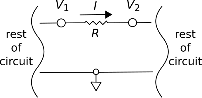
This method for calculating potential difference is often a bit awkward. To see why, consider an example from circuit theory, shown in Figure 5.5. In this example, consisting of a single resistor and a ground node, we’ve identified four quantities:
The resistance \(R\)
The current \(I\) through the resistor
The node voltage \(V_1\), which is the potential difference measured from ground to the left side of the resistor
The node voltage \(V_2\), which is the potential difference measured from ground to the right side of the resistor
Let’s say we wish to calculate the potential difference \(V_{21}\) across the resistor. There are two ways this can be done:
\(V_{21}=-IR\)
\(V_{21}=V_2-V_1\)
The advantage of the second method is that it is not necessary to know \(I\), \(R\), or indeed anything about what is happening between the nodes; it is only necessary to know the node voltages. The point is that it is often convenient to have a common datum – in this example, ground – with respect to which the potential differences at all other locations of interest can be defined. When we have this, calculating potential differences reduced to simply subtracting predetermined node potentials.
So, can we establish a datum in general electrostatic problems that works the same way? The answer is yes. The datum is arbitrarily chosen to be a sphere that encompasses the universe; i.e., a sphere with radius \(\to\infty\). Employing this choice of datum, we can use Equation 5.93 to define \(V({\bf r})\), the potential at point \({\bf r}\), as follows:
The electrical potential at a point, given by Equation 5.94, is defined as the potential difference measured beginning at a sphere of infinite radius and ending at the point \({\bf r}\). The potential obtained in this manner is with respect to the potential infinitely far away.
In the particular case where \({\bf E}\) is due to the point charge at the origin:
The principle of independence of path (Section 5.9) asserts that the path of integration doesn’t matter as long as the path begins at the datum at infinity and ends at \({\bf r}\). So, we should choose the easiest such path. The radial symmetry of the problem indicates that the easiest path will be a line of constant \(\theta\) and \(\phi\), so we choose \(d{\bf l}=\hat{\bf r}dr\). Continuing:
so
(Suggestion: Confirm that Equation 5.99 is dimensionally correct.) In the context of the circuit theory example above, this is the “node voltage” at \({\bf r}\) when the datum is defined to be the surface of a sphere at infinity. Subsequently, we may calculate the potential difference from any point \({\bf r}_1\) to any other point \({\bf r}_2\) as
and that will typically be a lot easier than using Equation 5.93.
It is not often that one deals with systems consisting of a single charged particle. So, for the above technique to be truly useful, we need a straightforward way to determine the potential field \(V({\bf r})\) for arbitrary distributions of charge. The first step in developing a more general expression is to determine the result for a particle located at a point \({\bf r}'\) somewhere other than the origin. Since Equation 5.99 depends only on charge and the distance between the field point \({\bf r}\) and \({\bf r}'\), we have
where, for notational consistency, we use the symbol \(q'\) to indicate the charge. Now applying superposition, the potential field due to \(N\) charges is
Substituting Equation 5.101 we obtain:
Equation 5.103 gives the electric potential at a specified location due to a finite number of charged particles.
The potential field due to continuous distributions of charge is addressed in Section 5.13.