9.1 The stretched string

We first consider the one-dimensional longitudinal vibrations that occur in a stretched string because of its elasticity. We start by modelling a set of \(n\) beads of mass \(m\) that are held together by springs with spring constant \(k\), as in Figure 9.1.

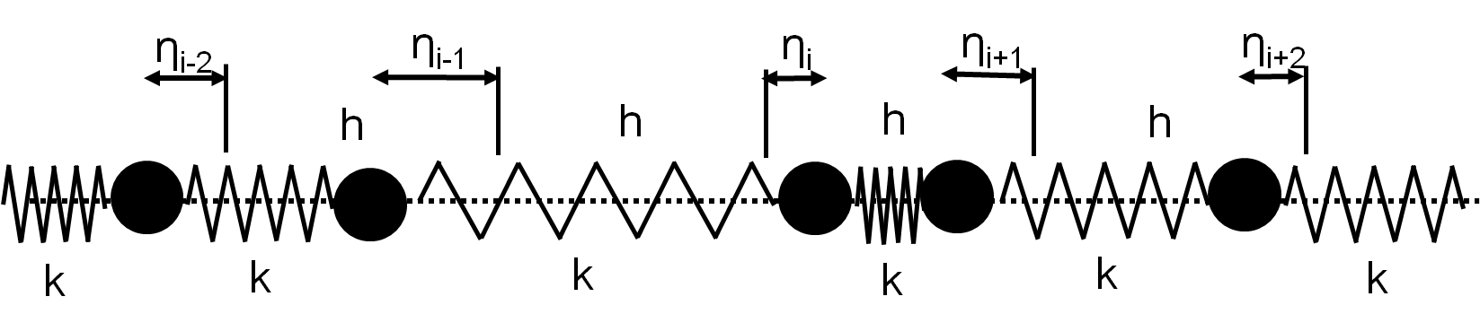
Long String — Figure 9.1A set of beads held together by springs to model longitudinal vibrations in a stretched string. At rest, the beads are separated by a distance \(h\).

The position of each bead is given by \(\eta_i\) and the string is fully described by the set of \(\eta_i\). The Lagrangian for the system is given by:

\begin{align} L=T-V=\sum_i^n \frac{1}{2}\left[m\dot\eta_i^2-k(\eta_{i+1}-\eta_i)^2\right] \tag{9.1}\end{align}

and the conditions that \(\eta_0=0\) and \(\eta_n=0\) (the ends of the string are fixed). We can apply the Euler-Lagrange equation to determine the equation of motion for \(\eta_i\):

\begin{align} \frac{d}{dt}\die{L}{\dot\eta_i}-\die{L}{\eta_i}&=0\\ \therefore m\ddot\eta_i-k(\eta_{i+1}-\eta_i)+k(\eta_i-\eta_{i-1})&=0 \tag{9.2}\end{align}

and this can be solved more generally with the method for coupled oscillators from Chapter ?.

In going from a discrete medium to a continuous medium, one can imagine making the masses as well as the distances between them infinitesimally smaller. As we move to a continuous system, the meaning of the \(\eta_i\) changes from the position of mass \(i\) to the amount of distance an element of the string at position \(i\) has been displaced. In fact, we can no longer use a discrete index, \(i\), to label the "particle" in the system. Rather, we should use a continuous variable, say \(x\), to label position along the string. We thus describe the position of the various mass elements along the string with a continuous function \(\eta(x)\). Recall, \(\eta\) is the generalized coordinate, not \(x\)! \(x\) is just a “label” for the generalized coordinate. Formally, \(\eta(x)\) is called a “field”.

Let us introduce, \(h\), as the distance between the masses on the string when they are at rest. To go from a discrete to a continuous system, we will let \(h\) go to zero. Introducing \(h\), we can re-write the Lagrangian as:

\begin{align} L=\sum_i^n h\frac{1}{2}\left[\frac{m}{h}\dot\eta_i^2-hk\left(\frac{\eta_{i+1}-\eta_i}{h}\right)^2\right] \tag{9.3}\end{align}

It is clear that the term \(\frac{m}{h}\) will become the mass per unit length of the string, \(\mu\). The term \(hk\) is Young’s modulus for the string, \(Y\). Recall Hooke’s Law for a continuous rod/string:

\begin{align} F=Y\lambda \tag{9.4}\end{align}

where \(F\) is the force required to stretch the rod by an amount \(\lambda\) per unit length (or conversely, for a given force \(F\), Hooke’s Law indicates how much the rod will stretch/contract per unit length). In the case of a discrete system, the contraction per unit length is \(\frac{\eta_{i+1}-\eta_i}{h}\), and so Hooke’s law would read:

\begin{align} F=k(\eta_{i+1}-\eta_i)=hk\left(\frac{\eta_{i+1}-\eta_i}{h}\right)=Y\lambda \tag{9.5}\end{align}

so that \(kh\) can indeed be identified with Young’s modulus. We thus have the Lagrangian:

\begin{align} L=\sum_i^n h\frac{1}{2}\left[\mu\dot\eta_i^2-Y\left(\frac{\eta_{i+1}-\eta_i}{h}\right)^2\right] \tag{9.6}\end{align}

In going to the limit of a continuous system, we have the following conditions:

\begin{align} i&\to x \\ \eta_i &\to \eta(x)\\ \eta_{i+1} &\to \eta(x+h)\\ \eta_{i+1}-\eta_i &\to \eta(x+h)-\eta(x) \to d\eta\\ h&\to dx \\ \sum_i^n h &\to \int \,dx \tag{9.7}\end{align}

So that the Lagrangian is given by:

\begin{align} L&=\int \frac{1}{2}\left[\mu\left(\frac{d\eta}{dt}\right)^2-Y\left(\frac{d\eta}{dx}\right)^2\right]\,dx\\ &=\int \mathcal{L} \,dx \tag{9.8}\end{align}

where we have introduced the “Lagrangian density”:

\begin{align} \mathcal{L}\equiv=\frac{1}{2}\left[\mu\left(\frac{d\eta}{dt}\right)^2-Y\left(\frac{d\eta}{dx}\right)^2\right] \tag{9.9}\end{align}

and we note that the field, \(\eta(x,t)\), is a function of \(x\) and \(t\). Rather than apply the variational principle to the Lagrangian, we can look at the equation of motion by converting the discrete version of the Euler-Lagrange equation that we had to the continuous version with the same replacements:

\begin{align} m\ddot\eta_i-k(\eta_{i+1}-\eta_i)+k(\eta_i-\eta_{i-1})&=0\\ \mu\ddot\eta_i-kh\frac{(\eta_{i+1}-\eta_i)-(\eta_i+\eta_{i-1})}{h^2}&=0\\ \mu\ddot\eta_i-Y\frac{1}{dx}\frac{(\eta_{i+1}-\eta_i)-(\eta_i-\eta_{i-1})}{dx}&=0\\ \mu\ddot\eta_i-Y\frac{1}{dx}\frac{(\eta(x+dx)-\eta(x))-(\eta(x)-\eta(x-dx))}{dx}&=0\\ \mu\ddot\eta_i-Y\frac{1}{dx}\left(\frac{d\eta}{dx}\bigr\rvert_{x+h}-\frac{d\eta}{dx}\bigr\rvert_x\right)&=0\\ \mu\frac{d^2\eta}{dt^2}-Y\frac{d^2\eta}{dx^2}&=0 \tag{9.10}\end{align}

which is the wave equation, with propagation speed:

\begin{align} v=\sqrt{\frac{Y}{\mu}} \tag{9.11}\end{align}

In this derivation, we did not actually apply the variational principles of mechanics. Rather, we took the Lagrangian and the result from the discrete case and made both equations continuous by taking the limit of small \(h\). Of course, we expect that the variational principle should give us the correct equation of motion from the Lagrangian density.