8.5 Action-angle variables

Action-angle variables are an extension to the Hamilton-Jacobi method, when the Hamiltonian does not depend on time. This formalism will allow us to determine certain fundamental frequencies of the system without explicitly solving the equations of motion. This method also allows one to transition from classical to quantum mechanics. Recall that in the case where the Hamiltonian does not depend on time, we can use Hamilton’s Characteristic function, \(W\) in lieu of \(S\):

\begin{align} S(q_i,\alpha_i,t)&=W(q_i,\alpha_i)-Et\\ p_i&=\die{W}{q_i}\\ H(q_i,\die{W}{q_i})&=E \tag{8.36}\end{align}

We will consider the case where \(W\) is “separable” (at least in some of the coordinates):

\begin{align} W(q_1,\dots, q_n,\alpha_i)=W_1(q_1,\alpha_i)+\dots +W_n(q_n,\alpha_i) \tag{8.37}\end{align}

that is, where the motion in each separable coordinate can be treated as independent from the others coordinates. The conjugate momentum for the separable coordinates are given by:

\begin{align} p_i&=\die{W_i(q_i, \alpha_1, \dots , \alpha_n)}{q_i}\end{align}

Furthermore, we will consider the case of “periodic’ motion. Two such cases are considered. First, “vibrations” where the coordinates and their momenta, \(p_i,q_i\), will, after a certain period of time, return to their original values. This is the case, for example, for a simple harmonic oscillator. Second, “rotations” where the momentum, \(p_i\), is periodic as a function of its generalized coordinate, \(q_i\). This is the case, for example, for a pendulum that has enough energy to “go over the top” (the angular position of the pendulum increases indefinitely with time and the momentum is periodic). The two cases are illustrated in phase space in Figure 8.1.

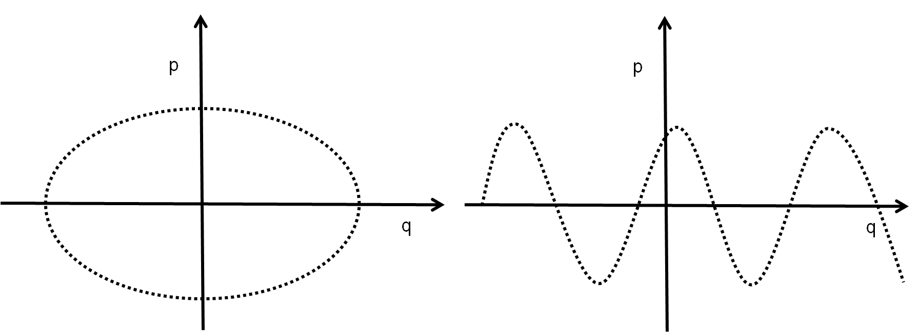
We start by introducing the “action-variables”, \(J_i\), obtained by integration over 1 period of the generalized coordinate:

\begin{align} J_i\equiv \oint p_idq_i \tag{8.39}\end{align}

There is one action variable per separable coordinate. Given the relations for the conjugate momenta for separable variables, we have:

\begin{align} J_i&=\oint p_idq_i\\ &=\oint \die{W_i(q_i, \alpha_1, \dots , \alpha_n)}{q_i} dq_i \end{align}

and the \(J_i\) thus only depend on the \(\alpha\), which are constants of the motion. The \(J_i\) are thus constants of the motion as well. We assume that the equations relating the \(J_i\) and \(\alpha_i\) are invertible:

\begin{align} J_i&=J_i(\alpha_1, \dots , \alpha_n)\\ \alpha_i&=\alpha_i(J_1, \dots, J_n) \tag{8.41}\end{align}

We can thus re-write Hamilton’s characteristic function, \(W\), and the Hamiltonian in terms of the \(J\) instead of the \(\alpha\):

\begin{align} W(q_i,\alpha_i)&\to W(q_i, J_i)\\ H(q_i,\die{W}{\alpha_i})&\to H(q_i,\die{W}{J_i})\\ S(q_i,\die{W}{\alpha_i})&\to W(q_i, J_i)-Et =W(q_i, J_i)-Ht \tag{8.42}\end{align}

In effect, we have chosen a new canonical transformation where \(J_i\) are the momenta, \(P_i\). In terms of the generating function \(S\), we have:

\begin{align} p_i&=\die{S}{q_i}\\ Q_i&=\die{S}{J_i} \tag{8.43}\end{align}

where \(S\) still satisfies the Hamilton-Jacobi equation. The new canonical momenta, \(J_i\), are thus still constants of motion, and we have:

\begin{align} P_i\equiv J_i&=\text{const.}\\ Q_i\equiv \beta_i&=\text{const.} \tag{8.44}\end{align}

We introduce the “angle variables”, \(w_i\):

\begin{align} w_i\equiv\die{W(q_1,\dots , q_n,J_1, \dots , J_n)}{J_i} \tag{8.45}\end{align}

and consider the constants \(\beta_i\) in terms of the angle variables:

\begin{align} \beta_i&=\die{S}{J_i}\\ &=\die{}{J_i}(W(q_i, J_i)-Ht)\\ &=w_i-\die{H}{J_i}t \tag{8.46}\end{align}

We write this as:

\begin{align} w_i=\beta_i+\nu_it \tag{8.47}\end{align}

where we have introduced the “frequency”, \(\nu_i\) (we call it frequency only because of its units for the moment):

\begin{align} \nu_i\equiv\die{H}{J_i} \tag{8.48}\end{align}

Now, assume that the system has a period of \(T_i\) for the ith degree of freedom (recall that we imposed that the system was periodic). In the amount of time \(T_i\), the angle variable will have changed by an amount:

\begin{align} \Delta w_i \equiv w_i(t=T_i)-w_i(t=0)=\nu_iT_i \tag{8.49}\end{align}

We can also calculate the amount that \(w_i\) changes as the system goes through one period:

\begin{align} \Delta w_i &=\oint dw_i\\ &=\oint \sum_j \die{w_i}{q_j}dq_j \\ &=\oint \sum_j \die{}{q_j}\die{W}{J_i}dq_j\\ &=\die{}{J_i}\oint \sum_j \die{W}{q_j}dq_j\\ &=\die{}{J_i}\oint \sum_j p_jdq_j\\ &=\die{}{J_i}\sum_j\oint p_jdq_j\\ &=\die{}{J_i}\sum_jJ_j\\ &=1 \tag{8.50}\end{align}

where we have used the definition of the angle variables, the fact that the conjugate momenta can be obtained from \(W\), and the definition of the action variables. Equating the two expressions for \(\Delta w_i\), it is clear that \(\nu_i\) is indeed the frequency with which the system is periodic in the ith degree of freedom:

\begin{align} \nu_i=\frac{1}{T_i} \tag{8.51}\end{align}

Although the derivation was not particularly intuitive, we have in fact derived a rather elegant result. Namely that for a periodic system, one can re-write the Hamiltonian in terms of the action variable and the derivative of the Hamiltonian with respect to that action variable is the frequency of the motion in the associated coordinate.

Example 8-6

Determine the frequencies of a two-dimensional simple harmonic oscillator with different spring constants in the two dimensions

The Hamiltonian for this system is written as:

\begin{align*} H=\frac{1}{2m}(p_1^2+p_2^2)+\frac{1}{2}k_1q_1^2+\frac{1}{2}k_2q_2^2 \end{align*}

and since it does not depend explicitly on time, is a constant of the motion, which we will call \(E\). The Hamilton-Jacobi equation is given by:

\begin{align*} \frac{1}{2m}\left(\die{W}{q_1}\right)^2+\frac{1}{2m}\left(\die{W}{q_2}\right)^2+\frac{1}{2}k_1q_1^2+\frac{1}{2}k_2q_2^2=E \end{align*}

Here, the variables \(q_1\) and \(q_2\) can be separated, and the Hamilton Jacobi equation written as two independent equations:

\begin{align*} W=W_1(q_1)+W_2(q_2)\\ \frac{1}{2m}\left(\frac{dW_1}{dq_1}\right)^2+\frac{1}{2m}\left(\frac{dW_2}{dq_2}\right)^2+\frac{1}{2}k_1q_1^2+\frac{1}{2}k_2q_2^2=E \end{align*}

Since the total is a constant, the terms depending on only one of the \(q\) must be a constant, so we can write:

\begin{align*} \frac{1}{2m}\left(\frac{dW_1}{dq_1}\right)^2+\frac{1}{2}k_1q_1^2=\alpha_1\\ \frac{1}{2m}\left(\frac{dW_2}{dq_2}\right)^2+\frac{1}{2}k_2q_2^2=\alpha_2 \end{align*}

where \(\alpha_1\) and \(\alpha_2\) are constants. Solving for the differentials, we can write:

\begin{align*} p_i=\frac{dW_i}{dq_i}=\sqrt{2m(\alpha_i-\frac{1}{2}k_iq_i^2)} \end{align*}

Consider expressing \(q_i\) using a new variable, \(\theta_i\), given by:

\begin{align*} q_i&=\sqrt{\frac{2\alpha_i}{k_i}}\sin\theta_i\\ \therefore dq_i&=\sqrt{\frac{2\alpha_i}{k_i}}\cos\theta_id\theta_i \end{align*}

This gives:

\begin{align*} p_i&=\sqrt{2m\left(\alpha_i-\frac{1}{2}k_i(\frac{2\alpha_i}{k_i}\sin^2\theta_i)\right)}\\ &=\sqrt{2m\alpha_i\cos^2\theta_i} \end{align*}

We are now set to evaluate the action variables:

\begin{align*} J_i&=\oint p_i dq_i\\ &=\oint \sqrt{2m\alpha_i\cos\theta_i^2} \sqrt{\frac{2\alpha_i}{k_i}}\cos\theta_id\theta_i\\ &=2\alpha_i\sqrt{\frac{m}{k_i}}\int_o^{2\pi} \cos^2\theta_i d\theta_i\\ &=2\pi\alpha_i\sqrt{\frac{m}{k_i}} \end{align*}

This is trivally inverted to get \(\alpha\) in terms of \(J\):

\begin{align*} \alpha_i=\frac{J_i}{2\pi}\sqrt{\frac{k_i}{m}} \end{align*}

We can now obtain the Hamiltonian in terms of the action variables:

\begin{align*} H&=\alpha_1+\alpha_2\\ &=\frac{1}{2\pi}\left(\sqrt{\frac{k_1}{m}}J_1+\sqrt{\frac{k_2}{m}}J_2\right) \end{align*}

The fundamental frequencies for the two degrees of freedom are thus:

\begin{align*} \nu_1&=\die{H}{J_1}=\frac{1}{2\pi}\sqrt{\frac{k_1}{m}}\\ \nu_2&=\die{H}{J_2}=\frac{1}{2\pi}\sqrt{\frac{k_2}{m}} \end{align*}

as expected.

Connection to Quantum Mechanics

The Hamiltonian description of classical mechanics is important as it is connected with Quantum Mechanics. In this section, we look at a few similarities between the two formalisms and how they are connected.

Recall a few key points about Quantum Mechanics:

In Quantum Mechanics, the state of a system is described by a wave function: \(|\psi>\)
Observables are obtained by operating on the wave function: \(\hat X|\psi>=x|\psi>\)
Operators do not, in general, commute: \(\hat X\hat Y|\psi>\neq\hat Y \hat X|\psi>\)
In the Heisenberg representation, the state vector (wave function) is constant in time and the operators change with time
In the time dependent Schrödinger representation, the operators are constant in time and the wave-function changes with time

Poisson brackets and commutators

You may have noticed a similarity between the use of Poisson Brackets in Classical Mechanics and Commutator relations in Quantum Mechanics. In fact, the connection between Classical and Quantum Mechanics can be made by the prescription that the Poisson Brackets be replaced with commutators:

\begin{align} \{U,V\}\to \frac{1}{i\hbar}[\hat U,\hat V] \tag{8.52}\end{align}

where \(\hbar\) is Planck’s constant divided by 2\(\pi\). Now, consider the evolution of a system in classical mechanics; in particular, recall how the time-variation of some quantity, \(F(q_i,p_i,t)\), is given by its Poisson Bracket with the Hamiltonian:

\begin{align} \frac{dF}{dt}=\{F,H\}+\die{F}{t} \tag{8.53}\end{align}

Now consider the prescription from equation 8.52 to go to Quantum Mechanics:

\begin{align} \frac{d\hat F}{dt}=\frac{1}{i\hbar}[\hat F,\hat H]+\die{\hat F}{t} \tag{8.54}\end{align}

This gives precisely the time evolution of a quantum mechanical operator in the Heisenberg formulation. This “Canonical Prescription” is the most general for going from Classical to Quantum Mechanics.

The Hamilton-Jacobi equation and the Schrödinger equation

Consider the time-dependent Schrödinger equation:

\begin{align} H(q_i,p_i,t)\psi&=i\hbar\die{\psi}{t}\\ p_i&=\frac{\hbar}{i}\die{}{q_i} \tag{8.55}\end{align}

and consider a solution of the form:

\begin{align} \psi&=A e^{\frac{i}{\hbar}S(q_i,t)}\\ \therefore\frac{\hbar}{i} \die{\psi}{q_i}&=\hbar\psi\die{S}{q_i}\\ \therefore i\hbar \die{\psi}{t}&=-\hbar\psi\die{S}{t} \tag{8.56}\end{align}

Substituting into the Schrödinger equation:

\begin{align} \left(H(q_i,\die{S}{q_i},t)+\die{S}{t}\right)\hbar\psi=0 \tag{8.57}\end{align}

Since \(\psi\) cannot vanish, we obtain the Hamilton-Jacobi equation:

\begin{align} H(q_i,\die{S}{q_i},t)+\die{S}{t}=0 \tag{8.58}\end{align}

There is thus a connection between the Hamilton-Jacobi equation and the Schrödinger equation. Quantum and classical mechanics meet in the limit where \(\hbar\to 0\). The function \(S\) is the phase of the wave-function. In the case where we separated out the energy term from \(S\), we are equivalently searching for stationary states in the quantum mechanics formulation.

Sommerfeld and Wilson prescription

The earliest prescription for going from Classical to Quantum Mechanics is due to Sommerfeld and Wilson who postulated that requiring that the action variables be quantized is a sufficient condition to obtain a quantum mechanical description:

\begin{align} J_i=\oint p_i dq_i=nh \tag{8.59}\end{align}

where \(n\) is an integer and \(h\) is Planck’s constant. Consider for example the simple harmonic oscillator, where we have explicitly calculated the action variable in Example 8-6:

\begin{align} J=2\pi\alpha\sqrt{\frac{m}{k}}=nh \tag{8.60}\end{align}

where we can identify \(\alpha\) with the energy. Writing this in terms of the energy, we have:

\begin{align} \alpha=E=n \frac{h}{2\pi}\sqrt{\frac{k}{m}}=n\hbar\omega \tag{8.61}\end{align}

which is the correct quantization for a simple harmonic oscillator (apart for the ground state).

Consider a particle in a central force field, described in polar coordinates, where we have seen that the momentum \(p_\phi\) is conserved and equal to the z-component of angular momentum, \(L_z\). The action variable is easily determined:

\begin{align} J_\phi=\oint p_\phi d\phi=\int_)^{2\pi}L_zd\phi=2\pi L_z \tag{8.62}\end{align}

Applying the Sommerfeld-Wilson quantization prescription, we find that:

\begin{align} L_z=n\hbar \tag{8.63}\end{align}

which is the correct quantization for the angular momentum along a specific direction. One should however note that in Classical Mechanics, the total momentum is also equal to \(L_z\) and one could be wrongly tempted to conclude that the total angular momentum is quantized in units of \(\hbar\).

Finally, consider the fact that the energy can be written in terms of the quantized action variables:

\begin{align} E=H(J_1,\dots, J_n)=H(n_1h,\dots,n_nh) \tag{8.64}\end{align}

And consider the change in energy when one of the action variables changes by one unit:

\begin{align} J_i\to J_i+h \tag{8.65}\end{align}

The change in energy of the system is:

\begin{align} \Delta E= H(J_1,\dots,J_i+h,\dots, J_n)-H(J_1,\dots,J_i,\dots, J_n) \tag{8.66}\end{align}

If we write the first term as a Taylor series (since \(h\) is small):

\begin{align} H(J_1,\dots,J_i+h,\dots, J_n)=H(J_1,\dots,J_i,\dots, J_n)+\die{H}{J_i}h \tag{8.67}\end{align}

hence:

\begin{align} \Delta E=\die{H}{J_i}h=\nu_i h \tag{8.68}\end{align}

where \(\nu_i\) is the frequency of the corresponding degree of freedom. It should be clear that this is exactly equivalent to the prescription for the Bohr atom.

It should be noted that the Sommerfeld-Wilson prescription is part of the "old quantum mechanics" and was derived in an ad-hoc fashion before a more self-consistent formulation was obtained by Schrödinger, Heisenberg, Dirac and others.