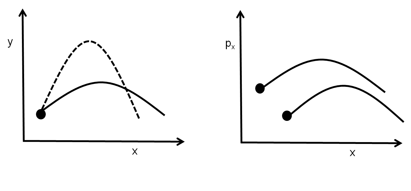
Recall that in the Lagrangian formalism, one can describe a system by specifying the value of its generalized coordinates in configuration space. In order to know the future (or past) development of the system, it is also necessary to specify the velocities. For example, a canon ball’s trajectory through (say, Cartesian) configuration space, depends on its velocity. In general, for a given starting position in configuration space, different initial velocities can lead to intersecting trajectories in configuration space (see Figure 7.1).
In the Hamiltonian formalism, the system is described by the generalized coordinates and by the generalized momenta. This can be viewed as a set of coordinates in “phase space”. The trajectory of the system through phase space is completely specified by the equations of motion. If the Hamiltonian does not change with time, the paths of different systems through phase space cannot intersect (this would mean that two systems with different positions (in configuration space) and momentum, following the same equations of motion, could end up at the same position and momentum). One can make the analogy with fluid dynamics, where the trajectories through phase space, for a system following a given Hamiltonian, are similar to the flow lines for a fluid (see Figure 7.1). Each trajectory corresponds to a particular value of the Hamiltonian. This fluid is called the “phase space fluid”.
Example 7-1
The Lagrangian is given by:
The Hamiltonian is thus:
Note that since \(L\) did not depend explicitly on time (and the kinetic energy is quadratic in the velocities, and the potential energy does not depend on velocity), \(H\) is equal to the total energy (\(T+V\)). Hamilton’s canonical equations are thus:
Since \(H\) is constant (\(=E\)), the Hamiltonian describes an ellipse in phase space:
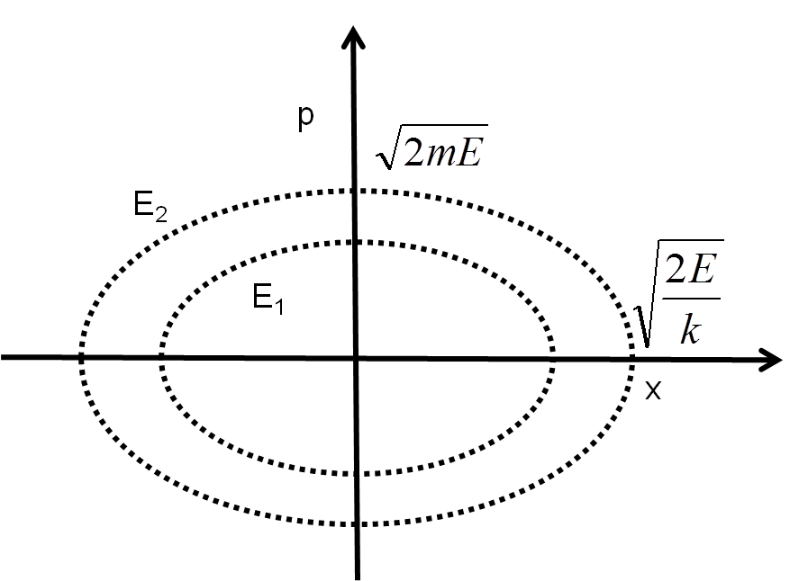
As the system evolves in time, it goes from a maximum value in \(x\) and zero momentum to a maximum value of momentum and zero value of \(x\), and so on. Momentum and position in phase space can easily be thought of on an equal footing.
Liouville’s theorem (although it was formulate by Gibbs and does not have much to do with Liouville) states that the phase space fluid acts like an incompressible fluid. That is, if you select a closed volume and let it evolve as the fluid moves in time, that total volume does not change with time. We know from fluid dynamics, that the divergence of the velocity field must be zero for an incompressible fluid. Indeed, consider the continuity equation for a fluid of density \(\rho\) and velocity field \(\vec v\):
If the density is constant (the fluid incompressible), then the divergence of the velocity vector is zero.
Treating the generalized momenta and the generalized coordinates as “regular” coordinates of a particle in configuration space, the velocity of that particle is given by a vector of dimension \(2n\):
where we have also substituted Hamilton’s canonical equations in the second equal sign.
If the divergence of the corresponding velocity field is zero:
which is equal to zero, since the partial derivatives commute. The velocity field in field space does indeed behave like an incompressible fluid.