6.1 Central Force Problem

One particle with 1 degree of freedom

Consider a simple system, with one (cartesian) degree of freedom and a potential of the form \(V(q_1)\), so that the Lagrangian is:

\begin{align} L=\frac{1}{2}m\dot{q}_1^2-V(q_1) \tag{6.1}\end{align}

This is called a “central force problem”, since it represents a particle of mass \(m\) with a force that is related to the distance from the origin and is directed towards or away from the origin. Example of such forces are Newtonian gravity, the Coulomb force, and the spring force. Since the Lagrangian does not explicitly depend on time, the total energy, \(E\) is conserved and is a constant. This allows the velocity to be determined from the position

\begin{align} E&=\frac{1}{2}m\dot{q}_1^2+V(q_1)\\ \dot{q}_1&=\sqrt{\frac{2}{m}(E-V(q_1))} \tag{6.2}\end{align}

Note that this implies that \(E-V(q_1)>0\), or the velocity would be imaginary.

The velocity equation can be integrated to get time as a function of position, and in principle, inverted to get position as a function of time:

\begin{align} \int_{t_0}^t dt=\int_{q_0}^{q_1(t)}\frac{dq_1}{\sqrt{\frac{2}{m}(E-V(q_1))}} \tag{6.3}\end{align}

Two particles and two degrees of freedom

Now consider two particles of mass \(m_1\), \(m_2\), each having a single degree of freedom and interacting with each other through a force that is related to the distance between the two particles. The total potential energy for the system would thus have a form \(V(q_2-q_1)\) and the Lagrangian is:

\begin{align} L=\frac{1}{2}m_1\dot{q}_1^2+\frac{1}{2}m_2\dot{q}_2^2-V(q_2-q_1) \tag{6.4}\end{align}

Again, the total energy of the system is a constant, since the Lagrangian does not depend explicitly on time. Interpreting \(q_i\) as the position of each particle along a q-axis, then the Lagrangian is invariant along translations in the q-direction:

\begin{align} q_1&\to q_1+\epsilon\tag{6.5}\\ q_2&\to q_2+\epsilon \tag{6.6}\end{align}

so there must be a conserved quantity:

\begin{align} Q&=\sum_ip_i\\ &=m_1\dot{q}_1+m_2\dot{q}_2 \tag{6.7}\end{align}

which is the total momentum in the q-direction.

Consider the following change of variables from (\(q_1\),\(q_2\)) to (\(r\), \(R\)):

\begin{align} r&\equiv q_2-q_1\\ R&\equiv \frac{m_1}{m_1+m_2}q_1+\frac{m_2}{m_1+m_2}q_2\\ M&\equiv m_1+m_2\\ \mu&\equiv \frac{m_1m_2}{m_1+m_2} \tag{6.8}\end{align}

where \(R\) is the coordinate of the center of mass, and \(\mu\) is called the “reduced mass”.

Example 6-1

Invert the transformation equations 6.8 for \(q_1\) and \(q_2\) to obtain the kinetic energy in terms of \(r\) and \(R\).

We have:

\begin{align*} R&=\frac{1}{m_1+m_2}(m_1q_1+m_2q_2)\nonumber\\ &=\frac{1}{m_1+m_2}(m_1q_1+m_2(q_1+r))\nonumber\\ &=\frac{m_2}{m_1+m_2}r+q_1\nonumber\\ \therefore q_1&=R-\frac{m_2}{m_1+m_2}r\nonumber\\ \therefore q_2&=R+\frac{m_1}{m_1+m_2}r\nonumber\\ \end{align*}

The total kinetic energy is thus:

\begin{align*} \frac{1}{2}m_1\dot{q_1}^2+\frac{1}{2}m_2\dot{q_2}^2&=\frac{1}{2}m_1(\dot{R}-\frac{m_2}{m_1+m_2}\dot{r})^2+\frac{1}{2}m_2(\dot{R}+\frac{m_1}{m_1+m_2}\dot{r})^2\nonumber\\ &=\frac{1}{2}m_1(\dot{R}^2-2\frac{m_2}{m_1+m_2}\dot{R}\dot{r}+\frac{m_2^2}{(m_1+m_2)^2}\dot{r}^2)+\frac{1}{2}m_2(\dot{R}^2+2\frac{m_1}{m_1+m_2}\dot{R}\dot{r}+\frac{m_1^2}{(m_1+m_2)^2}\dot{r}^2)\nonumber\\ &=\frac{1}{2}m_1(\dot{R}^2+\frac{m_2^2}{(m_1+m_2)^2}\dot{r}^2)+\frac{1}{2}m_2(\dot{R}^2+\frac{m_1^2}{(m_1+m_2)^2}\dot{r}^2)\nonumber\\ &=\frac{1}{2}(m_1+m_2)\dot{R}^2+\frac{1}{2}\frac{m_1m_2^2+m_2m_1^2}{(m_1+m_2)^2}\dot{r}^2\nonumber\\ &=\frac{1}{2}(m_1+m_2)\dot{R}^2+\frac{1}{2}m_1m_2\frac{m_1+m_2}{(m_1+m_2)^2}\dot{r}^2\nonumber\\ &=\frac{1}{2}M\dot{R}^2+\frac{1}{2}\mu\dot{r}^2 \end{align*}

In terms of the new coordinates, the Lagrangian is then:

\begin{align} L&=\frac{1}{2}M\dot{R}^2+\frac{1}{2}\mu\dot{r}^2-V(r)\end{align}

The \(R\) coordinate is cyclic, and the corresponding momentum:

\begin{align} P=M\dot{R} \tag{6.10}\end{align}

corresponding to the momentum of the whole system is conserved. The kinetic energy term from the center of mass is thus a constant added to the Lagrangian and does not influence the equations of motion; we can thus ignore it:

\begin{align} L&=\frac{1}{2}\mu\dot{r}^2-V(r)\end{align}

where we have effectively reduced the problem to an equivalent problem with one degree of freedom and the reduced mass.

Two particles and three dimensional motion

Let us know consider the general problem of two particles of mass \(m_1\) and \(m_2\), with position vectors \(\vec{r}_1\) and \(\vec{r}_2\) and a potential energy of the form \(V(\vec{r}_2-\vec{r}_2)\). The Lagrangian is:

\begin{align} L=\frac{1}{2}m_1\dot{\vec{r}}_1^2+\frac{1}{2}m_2\dot{\vec{r}}_2^2-V(\vec{r}_2-\vec{r}_1) \tag{6.12}\end{align}

Again, we can introduce new coordinates and the reduced mass:

\begin{align*} \vec{r}&\equiv \vec{r}_2-\vec{r}_1\nonumber\\ \vec{R}&\equiv \frac{m_1}{m_1+m_2}\vec{r}_1+\frac{m_2}{m_1+m_2}\vec{r}_2\nonumber\\ \mu&\equiv \frac{m_1m_2}{m_1+m_2}\nonumber\\ \therefore \vec{r}_1&=\vec{R}-\frac{m_2}{m_1+m_2}r\nonumber\\ \therefore \vec{r}_2&=\vec{R}+\frac{m_1}{m_1+m_2}r\nonumber\\ \end{align*}

The algebra to obtain the kinetic energy in the new coordinates is the same as in the previous section, and the Lagrangian can be written as:

\begin{align} L&=\frac{1}{2}\mu\dot{\vec{r}}^2-V(\vec{r})\end{align}

where we have used the fact that the total momentum is a constant of the motion:

\begin{align} P=M\dot{\vec{R}} \tag{6.14}\end{align}

Thus, in 3-dimensional space, the problem of two particles acting on each other through a central force (6 degrees of freedom) can be reduced to an equivalent problem with 1 particle acted on by a central force directed at the origin (3 degrees of freedom). As origin, we use the center of mass of the two particles, with a coordinate system that is co-moving with the center of mass.

Since space is homogeneous, the potential cannot depend on the actual direction of \(\vec{r}\) and should only depend on its magnitude. Indeed, if two particles acting on each other through a central potential (e.g. Coulomb force), the orientation in space of the particles will not matter. It is thus natural to describe the system using spherical coordinates, \(r\), \(\theta\), \(\phi\), with the Lagrangian:

\begin{align} L=\frac{1}{2}\mu(\dot{r}^2+r^2\dot{\theta}^2+r^2\sin^2\theta\dot{\phi}^2)-V(r) \tag{6.15}\end{align}

The Lagrangian is invariant under rotations of the coordinate system, thus the angular momentum in each direction is conserved. Since the total angular momentum is conserved, the motion must be constrained to the place perpendicular to the total angular momentum. We thus choose to orient our coordinate system such that the polar axis points in the direction of the total angular momentum. The angle \(\theta\) will thus be \(\frac{\pi}{2}\) and constant. The Lagrangian thus simplifies even further to:

\begin{align} L=\frac{1}{2}\mu(\dot{r}^2+r^2\dot{\phi}^2)-V(r) \tag{6.16}\end{align}

The coordinate \(\phi\) is cyclic, and the corresponding generalized momentum is conserved:

\begin{align} p_\phi&=\mu r^2\dot\phi=l\\ \therefore \dot\phi&=\frac{l}{r^2\mu} \tag{6.17}\end{align}

Recall, this does not mean that \(\dot\phi\) is constant, only that it can be determined from a constant and from \(r\). The constant, \(l\), is obviously angular momentum. We can thus write the Lagrangian as:

\begin{align} L=\frac{1}{2}\mu\dot{r}^2+\frac{l^2}{2\mu r^2}-V(r) \tag{6.18}\end{align}

Since the middle term depends only \(r\), we can introduce an “effective potential”, \(V_{eff}\)

\begin{align} V_{eff}\equiv V(r)+\frac{l^2}{2\mu r^2} \tag{6.19}\end{align}

and the Lagrangian is given by:

\begin{align} L=\frac{1}{2}\mu\dot{r}^2-V_{eff}(r) \tag{6.20}\end{align}

and we have again reduced the problem to a single degree of freedom!

Consider the force that arises from the effective potential:

\begin{align} F_r&=-\die{V_{eff}}{r}\\ &=-\die{V(r)}{r}-\die{}{r}\frac{l^2}{2\mu r^2}\\ &=-\die{V(r)}{r}-\die{}{r}\frac{1}{2}\mu r^2\dot\phi^2\\ &=-\die{V(r)}{r}+\mu r\dot\phi^2\end{align}

The second term (which we added) is in fact the apparent centrifugal force, trying to push the “particle” outwards (recall that we are actually modeling two particles in 3 dimensions!). This apparent force is zero if \(\dot\phi\) is zero.

Finally, conservation of energy allows us to solve for \(r(t)\) by inverting the solution to:

\begin{align} t=\int_{r_0}^{r(t)}\frac{dr}{\sqrt{\frac{2}{\mu}(E-V_{eff}(r))}} \tag{6.22}\end{align}

Using analytic mechanics we have thus been able to understand a lot about a system with a central force, without solving any differential equations and without even knowing the form of the force (or potential)! We have found that:

A system of two particles interacting through a central force in three dimensions can be reduced to an equivalent system with 1 degree of freedom
Energy is conserved (since \(L\) does not depend on t)
Motion is confined to a plane (angular momentum is conserved)

Qualitative characteristics of orbits

Let us make a few more general observation on the dynamics of a particle subject to a central force. We start by considering a potential that gives an attractive inverse-square force law (such as gravity):

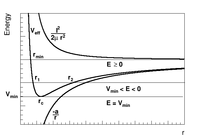
\begin{align} V(r)&=\frac{-a}{r}\\ \therefore V_{eff}(r)&= \frac{-a}{r}+\frac{l^2}{2\mu r^2} \tag{6.23}\end{align}

The corresponding \(V_{eff}(r)\) is sketched in figure 6.1 for a particular value of the angular momentum and \(a\). Three possible cases for the energy are also shown:

If the energy is larger than zero, all possible values of \(r>r_{min}\), are allowable. \(r_{min}\) corresponds to the case where \(V_{eff}=E\). If the particle arrives from infinity, it will drift towards \(r=0\) until it reaches \(r_{min}\) where it will experience a repulsive force that pushes it back out from the center of mass. This repulsive force is from the conservation of angular momentum. The only case that the particle can fall into the center of mass is if \(l=0\), that is, there is no angular momentum with respect to the center of mass (the impact parameter is zero).
If the energy is less than zero, but bigger that the minimum of \(V_{eff}\), the particle is constrained to be between two circles of radius \(r_1\) and \(r_2\). This does not necessarily mean that the orbit is “closed”, only that the trajectory is constrained between two circles.
If the energy is exactly \(V_{min}\) then the particle is constrained to a specific radius, \(r_c\). In this case, the orbit is necessarily closed and circular. The minimum of \(V_{eff}\) occurs when:

\begin{align} \frac{dV_{eff}}{dr}&=0\\ \frac{a}{r^2}&=\frac{l^2}{\mu r^3}\\ \frac{a}{r^2}&=\mu r \dot\phi^2 \tag{6.24}\end{align}

which is precisely the requirement that the centripetal force (\(\frac{a}{r^2}\)) equal mass times centripetal acceleration. This corresponds to a radius \(r_c\) and energy \(E=V_{min}\) given by:

\begin{align} r_c&=\frac{l^2}{a\mu}\\ V_{min}&=V_{eff}(r_c)=-\frac{a}{r_c}+\frac{l^2}{2\mu r_c^2}=-\frac{a^2\mu}{2l^2} \tag{6.25}\end{align}

The value of the angular momentum and the initial value of the radius will determine the ultimate trajectory of the particles. Note that the kinetic energy of the particle (in the radial direction) is always equal to the distance between \(E\) and \(V_{eff}\):

\begin{align} T_r(r)=\frac{1}{2}\mu\dot r^2=E-V_{eff}(r) \tag{6.26}\end{align}

which is zero for the circular orbit.

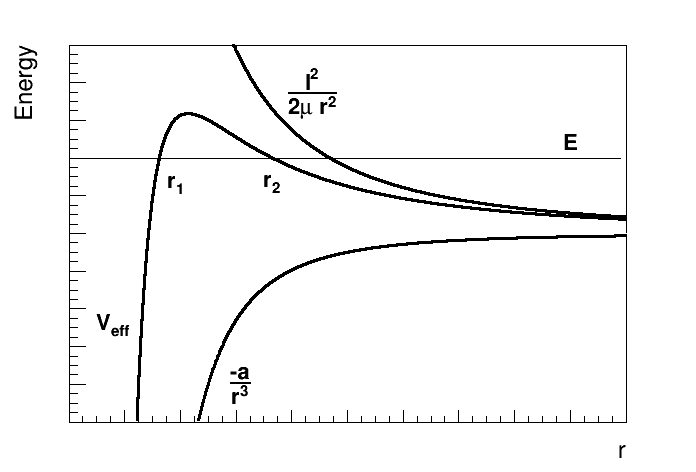
Central Potential labels — Figure 6.1Effective potential for the case where \(V(r)=-ar^{-1}\). The horizontal lines show three possible values for the energy.

Consider a potential that gives an attractive inverse-fourth force law:

\begin{align} V(r)&=\frac{-a}{r^3}\\ \therefore V_{eff}(r)&= \frac{-a}{r^3}+\frac{l^2}{2\mu r^2} \tag{6.27}\end{align}

The effective potential is sketched in Figure 6.2, along with a possible energy \(E\). For this particular case of energy choice, the motion will depend on the initial condition. If the particle started with a radius less than \(r_1\) the motion will be bound and constrained to a radii smaller than \(r_1\). These orbits will pass through the center of mass. In the case where the initial radius was bigger than \(r_2\), the particle will experience a repulsive force and never access radii smaller than \(r_2\). Of course, the repulsive force, is again the apparent centrifugal force.

Central Potential fourth — Figure 6.2Effective potential for the case where \(V(r)=-ar^{-3}\).

Determining the equation of the orbit

For certain potentials, it is possible to solve for the equation of the orbit. Starting from the Lagrangian:

\begin{align} L=\frac{1}{2}\mu\dot{r}^2+\frac{l^2}{2\mu r^2}-V(r) \tag{6.28}\end{align}

We know that conservation of energy gives

\begin{align} \frac{1}{2}\mu\dot{r}^2+\frac{l^2}{2\mu r^2}+V(r)&=E\end{align}

This can be integrated to give r(t). However, we really are interested in obtaining \(r(\phi)\). Using the Chain Rule, we can convert the above differential equation from an equation for \(r(t)\) to an equation for \(r(\phi)\). Consider:

\begin{align} \frac{dr}{dt}=\frac{dr}{d\phi}\dot\phi \tag{6.30}\end{align}

We can use the conservation of angular momentum:

\begin{align} \dot\phi&=\frac{l}{r^2\mu}\\ \therefore \frac{dr}{dt}&=\frac{dr}{d\phi}\frac{l}{r^2\mu}\\ \therefore \frac{1}{2}\mu\left( \frac{dr}{d\phi}\frac{l}{r^2\mu} \right)^2+\frac{l^2}{2\mu r^2}+V(r)&=0\\ \frac{l^2}{2\mu}\left[\frac{1}{r^4}\left( \frac{dr}{d\phi} \right)^2+\frac{1}{r^2}\right]+V(r)&=E \tag{6.31}\end{align}

Let us now introduce a substitution of variables:

\begin{align} u&\equiv \frac{1}{r}\\ \therefore \frac{du}{d\phi}&=\frac{du}{dr} \frac{dr}{d\phi}= -\frac{1}{r^2} \frac{dr}{d\phi} \\ \therefore \frac{dr}{d\phi}&=-r^2\frac{du}{d\phi} \tag{6.32}\end{align}

The differential equation then becomes:

\begin{align} \frac{l^2}{2\mu}\left[\left( \frac{du}{d\phi} \right)^2+u^2\right]+V(\frac{1}{u})&=E \tag{6.33}\end{align}

Let us assume that the potential has the following form:

\begin{align} V(r)=ar^{-n} \tag{6.34}\end{align}

Careful! This is a different definition than in the previous section where we had forced \(a\) to be positive. Here, we allow a to be positive (repulsive force) or negative (attractive force). The differential equation is then:

\begin{align} \left[\left( \frac{du}{d\phi} \right)^2+u^2\right]+\frac{2\mu}{l^2}au^n&=\frac{2\mu}{l^2}E \tag{6.35}\end{align}

again, we can write this as an integral:

\begin{align} \int_{\phi_0}^\phi d\phi&=\int_{u_0}^u \frac{du}{\sqrt{\frac{2\mu}{l^2}E-\frac{2\mu}{l^2}au^n-u^2}}\\ &=-\int_{r_0}^r \frac{dr}{r^2\sqrt{\frac{2\mu}{l^2}E-\frac{2\mu}{l^2}ar^{-n}-\frac{1}{r^2}}} \tag{6.36}\end{align}

where we have used the fact that \(du=-\frac{1}{r^2}dr\). This can be integrated analytically for certain values of \(n\).

The case of gravity (“Kepler’s problem”)

Let us solve specifically the case of two masses \(m_1\) and \(m_2\) interacting with gravity:

\begin{align} V(r)&=ar^{-n}=-\frac{Gm_1m_2}{r}\\ a&=-Gm_1m_2\\ n&=1 \tag{6.37}\end{align}

The differential equation for \(r(\phi)\) is thus:

\begin{align} \left[\left( \frac{du}{d\phi} \right)^2+u^2\right]-\frac{2\mu}{l^2}au&=\frac{2\mu}{l^2}E \tag{6.38}\end{align}

Let us introduce a constant, \(\alpha\):

\begin{align} \alpha&\equiv\frac{l^2}{a\mu}\\ \therefore \left[\left( \frac{du}{d\phi} \right)^2+u^2\right]-\frac{2}{\alpha}u&=\frac{2E}{a\alpha} \tag{6.39}\end{align}

We now add \(\frac{1}{\alpha^2}\) to both sides:

\begin{align} \left[\left( \frac{du}{d\phi} \right)^2+u^2\right]-\frac{2}{\alpha}u+\frac{1}{\alpha^2}&=\frac{2E}{a\alpha}+\frac{1}{\alpha^2}\end{align}

We introduce a new function, \(f\), and a new constant \(K\):

\begin{align} f(\phi)&\equiv u(\phi)-\frac{1}{\alpha}\\ \left(\frac{df}{d\phi}\right)^2&=\left(\frac{du}{d\phi}\right)^2\\ f^2&=u^2-2u\frac{1}{\alpha}+\frac{1}{\alpha^2}\\ K^2&\equiv\frac{1}{\frac{2E}{a\alpha}+\frac{1}{\alpha^2}} \tag{6.41}\end{align}

The differential equation becomes:

\begin{align} K^2\left[\left( \frac{df}{d\phi} \right)^2+f^2\right]&=1\\ \left[\left( \frac{dKf}{d\phi} \right)^2+(Kf)^2\right]&=1\\ \left[\left( \frac{dg}{d\phi} \right)^2+g^2\right]&=1\end{align}

where we have introduced a new function \(g(\phi)=Kf(\phi)\). We can identify \(g\) with a trigonometric function, let’s choose:

\begin{align} g&=\cos\phi \tag{6.43}\end{align}

and the differential equation is obviously satisfied by the trigonometric identity \(\cos^2+\sin^2=1\). The solution is thus:

\begin{align} f(\phi)&=\frac{1}{K}\cos(\phi)= u(\phi)-\frac{1}{\alpha}\\ u(\phi)&=\frac{1}{K}\cos(\phi)+\frac{1}{\alpha}\\ &=\sqrt{\frac{2E}{a\alpha}+\frac{1}{\alpha^2}}\cos(\phi)+\frac{1}{\alpha}\\ &=\frac{1}{\alpha}\sqrt{\frac{2E\alpha}{a}+1}\cos(\phi)+\frac{1}{\alpha}\end{align}

Introducing the quantity, \(e\):

\begin{align} e^2&\equiv \frac{2E\alpha}{a}+1\\ \frac{1}{r}&=\frac{e}{\alpha}\cos(\phi)+\frac{1}{\alpha}\end{align}

Finally, multiplying by \(r\alpha\), we obtain the equation for a conical curve of eccentricity \(e\) in polar coordinates:

\begin{align} r(e\cos\phi+1)&=\alpha\end{align}

which is what we expect from Kepler’s laws. Note that we only considered the shape of the trajectory, so we ignored the initial condition on \(r\) or \(\phi\) when performing the integral. If we need to obtain the equations for \(r\) as a function of time, it would be important to include the initial condition of \(\phi\) and replace \(\phi\to\phi-\phi_0\).

Recall the properties of the eccentricity, \(e\), for conical curves:

\(e=0\) corresponds to a circle centered on the origin
\(0\leq e \leq 1\) corresponds to an ellipse with a focus at the origin
\(e=1\) corresponds to a parabola
\(e>1\) corresponds to a hyperbola

We can relate this to our earlier qualitative comments about the the orbits, based on the energy:

\begin{align} e^2&=\frac{2E\alpha}{a}+1 \\ &=E\frac{2l^2}{a^2\mu}+1\\ \therefore E&=\frac{\mu a^2}{2l^2}(e^2-1) \tag{6.47}\end{align}

An energy of zero thus results in a parabolic trajectory (\(e=1\)). The circular orbit (\(e=0\)) is given by:

\begin{align} E&=-\frac{\mu a^2}{2l^2}\end{align}

which is the result we obtained earlier. If \(e\) is bigger than 1, then the energy is positive and the orbit is unbound (a hyperbola). If \(e\) is less than 1, then the energy is negative and the orbit is bound (an ellipse).