The Lagrangian has several properties that we explore here.
Invariance with respect to point transformations
Coordinate transformations \(q\to q'\) can generally be called “contact transformations” and written in the form:
The functional forms of the \(q_i'\) must satisfy certain conditions to be allowable (e.g. continuous, differentiable, non-zero Jacobian). When the transformation does not depend on the derivatives (velocities), the transformation is called a “point transformation”. A point transformation is a mapping of a space onto a different space and requires that each point be mapped onto a unique point in the mapped spaced. Thus, points that are near each other remain near each other in the mapped space. A common mapping would be to change coordinates from cartesian to polar coordinates:
In this case, a square in cartesian space does not map into a square in the space of polar coordinates, as seen in Figure 4.4. Other properties are however preserved. If two lines do not intersect in one space, then they won’t intersect in the other space either. As one considers points that are closer together their geometrical properties in the mapped space become more similar. For example, a very small square in cartesian coordinates, maps into something that almost looks like a square in polar coordinates.
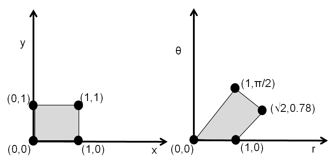
Lagrange’s equations determine the evolution of a system in n-dimensional configuration space (the space of the \(n\) generalized coordinates). One can extend the configuration space by one dimension, to include time as well. The evolution of a system is then a curve in the n+1 dimensional space, and the Lagrange equations determine the shape of that curve given that the end points are fixed. Through a point transformation, that curve will map to a curve that also follows the Lagrange equations in the mapped space (since infinitesimals are preserved through a point transformation). Thus, the Lagrangian description of motion is invariant under point transformations. That is, even though the actual functional form of the Lagrangian is different under a transformation of the coordinates, it invariably describes the same physical process.
This means that we are generally free to choose the set of generalized coordinates for which to describe the system (it makes sense that the Lagrangian description not depend on the choice of coordinates). This is one of the great powers of the Lagrangian method. One should be a little careful here, as describing a system using a moving frame of reference is still an acceptable point transformation. In Special Relativity, we know that the description of time depends on the relative speed of the two reference frames. We will see later that in the case of Special Relativity, we have to treat time the same way as one of the coordinates, and time will also be allowed to transform from one coordinate system to the other. With that modification, the Lagrangian will be truly independent of the coordinate system (provided they are related to an inertial system through a point transformation).
Example 4-6
The Lagrangian in cartesian coordinates is:
The equations of motion from Lagrange’s equation are easily seen to be:
In polar coordinates, we have:
The equations of motion from Lagrange’s equation are:
Thus we find that \(\dot{\theta}\) is a constant, and the rate of change of \(r\) is such that the particle will go in a straight line (when projected on the \(r\)-\(\theta\) plane).
Addition of Lagrangians
The Lagrangians of different particles (or different systems) are additive. That is, given a Lagrangian \(L_A\) for a system \(A\) and a Lagrangian, \(L_B\), for a system \(B\), the entire system \(A+B\) can be described by the Lagrangian \(L=L_A+L_B\). This is easily shown by the additive properties of derivatives in the Euler-Lagrange equations:
Multiplication of the Lagrangian by a constant
The equations of motions are not affected if the Lagrangian is multiplied by an overall constant:
For a free particle, multiplication of the Lagrangian by a constant is analogous to changing the units of mass.
Addition of a total time derivative
Similarly, the Lagrangian is un-affected if one adds to the Lagrangian a function that is a total time-derivative, \(\frac{df}{dt}\):
When taking the variation of the action, the last two terms will vanish, since the end points of the \(L\) curve in configuration space are fixed. Of course, the Lagrangian is unchanged if a constant term is added to the Lagrangian (this can be thought of as a change in the absolute value of the potential energy).
Lagrangian does not explicitly depend on time
If the Lagrangian is independent of time, the Euler-Lagrange equations simplify, as we saw in the case of equation 2.57, when we looked at the calculus of variations. In the case where \(L\) does not explicitly depend on time, the Euler-Lagrange equations imply that:
where \(h\) is a constant. In fact, we will see that \(h\) is related to the “Hamiltonian” of the system. \(h\) is called the “Jacobi integral” and can be calculated whether or not it is a constant by using the second equation. It is only a constant when \(L\) does not explicitly depend on time:
One can in general re-write \(h(q_i, \dot{q}_i, t)\) and replace \(\dot{q}_i\to p_i\), and obtain a new function, \(H(q_i,p_i,t)\) which is called the Hamiltonian.
Equation 4.33 is the general form for the quantity \(h\) that is conserved if \(L\) does not explicitly depend on time. If we make the following, further, assumptions:
The kinetic energy is of the form \(T=\frac{1}{2}\sum_{j=1}^n\sum_{k=1}^na_{jk}\dot{q}_j\dot{q}_k\), that is, quadratic in the velocities. Note that \(a_{jk}=a_{kj}\), since these are partial derivatives of the generalized coordinates.
The potential energy, \(V\), does not depend explicitly on the velocities (\(\frac{\partial V}{\partial\dot{q}_i}=0\)).
The we have:
and we see that, in the case where \(L\) does not explicitly depend on time, \(T\) is quadratic in the velocities, and \(V\) does not depend on velocities, the total energy of the system, \(T+V\), is the conserved quantity \(h\). This situation leads to a particularly simple treatment for problems with 1 degrees of freedom, as the solution for the equation of motion, \(q(t)\) can always be written out as an integral:
which can then be inverted to obtain \(q(t)\).
Example 4-7
The system has one degree of freedom, and we will use \(x\) as the generalized coordinate. The Lagrangian is independent in time, quadratic in \(x\), and the potential does not depend on velocity:
The total energy, \(h=T+V=\frac{1}{2}kx_0^2\) is thus conserved. We can use equation 4.36 to obtain the period, \(t\), for the motion (noting that the period is four time the time to go from \(x_0\) to \(0\)):
Cyclic coordinates - Lagrangian does not depend on a specific coordinate
In some cases, the Lagrangian does not depend explicitly on all of the generalized coordinates. The Lagrangian will still depend implicitly on those coordinates through their velocities in the kinetic energy. We call those coordinates that do not explicitly appear in the Lagrangian “cyclic”, or “ignorable”, or “kinosthenic”. In this case, the equations of motion also simplify for those coordinates:
where \(p_i\) are constants for each of the cyclic coordinates.
Example 4-8
The Lagrangian for a particle in a gravitational field is given by:
We can see that the coordinates \(x\) and \(y\) are cyclic. Thus the following quantities are conserved:
which we can identify with the linear momentum, which should be conserved in the two directions not affected by gravity.
Also note that \(L\) does not explicitly depend on time. We can thus write the following equation for the conserved quantity, \(h\):
We see that the constant quantity, \(h\), is in fact the total energy of the system, \(E\). We recover the observation that the total energy of the system is conserved if the Lagrangian does not depend explicitly on time. Using the constants of the motion (\(p_x\), \(p_y\), \(h\)), we can easily write the equations of motion:
As a flavour of what is to come, let’s consider the quantities:
and it is clear that these are just the component of the linear momentum. Furthermore, we can write \(H\) as a function of only \(p_i\) and \(q_i\), without using the velocities, \(\dot{q}_i\):
In principle then, the system is completely described by the new coordinates (momentum and position). Finally, note that the Lagrangian does not depend explicitly on \(x\) or \(y\). We saw in Equation 4.37 that this results in \(p_x\) and \(p_y\) being constants. Of course, this makes sense, as the linear momentum is constant except in the direction acted upon by gravity.