We saw in the previous chapter, Example 3-7, that for a particle that is subject to a conservative force (a force that can be obtained from the gradient of the potential energy), D’Alembert’s principle leads to a particularly elegant way of solving for the equations of motion. One needs only write the Lagrangian, \(L=T-V\), given by the kinetic minus the potential energy of the particle, and find the condition for the action, \(S=\int Ldt\) to be stationary. Let’s revisit that example. First, let’s motivate the statement that \(V\) is the potential energy. If we have a force, \(F\), that is given by the negative of the gradient of \(V\):
which is precisely the definition of the potential energy (the negative of the work done by the force).
We are thus convinced that for a conservative force acting particle, \(T-V\), really is the difference between kinetic and potential energy (sometimes called the “excess kinetic energy”).
where the sum over \(i\) is over all the forces on the particle. For a single particle, this can be the broken up into the sum of \(N_C\) conservative forces, \(\vec{F}_i^{C}\), plus the sum of \(N_{NC}\) non-conservative forces, \(\vec{F}_i^{NC}\):
where we have introduced a potential energy, \(V_i\), for each conservative force, and the total potential energy, \(V\), as the sum of the potential energies. Note that the potential energy can now be expressed in terms of the generalized coordinates. Writing D’Alembert’s principle, we get:
which is a general version of D’Alembert’s principle that includes non-conservative forces. This does require that the system be holonomic, that is, the generalized coordinates are independent of each other (since this result depends on being able to take variations of the generalized coordinates independently). Introducing the Lagrangian, \(L=T-V\), we get:
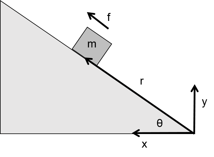
Determine the equation of motion for a block of mass, \(m\), that is sliding with friction down an inclined slope of angle \(\theta\). The friction force has a magnitude \(f\).
Figure 4.1Block sliding with friction
We start by identifying that there is only 1 degree of freedom, and we choose the variable \(r\) as the generalized coordinate (the distance from the block to the origin in Figure 4.1). The coordinate transformations are thus:
giving us back D’Alembert’s equation in generalized coordinates. Without loss of generality, we will let \(V\) stand for any generalized potential and the Lagrangian \(L\) will include the potentials associated with any monogenic forces.
Example 4-2
A charge, \(e\), is moving with a velocity, \(\vec{v}\), in a region of electric field, \(\vec{E}\) and magnetic field \(\vec{B}\) Both fields are free to vary in space and time. Show that a generalized potential given by \(V=e\phi-e\vec A\cdot \vec v \) (where \(phi\) is the electric potential, \(\vec A\) is the vector potential, and \(\vec v\) is the velocity vector) results in the Lorentz force and write out the Lagrangian for the particle.
Since the particle is moving in free space, we can use Cartesian coordinates as the generalized coordinates. In general, an electric and magnetic field are described by a scalar electric potential, \(\phi\), and the vector potential, \(\vec{A}\), where
where the first term is clearly the electrical potential energy and the second term is velocity dependent. This generalized potential gives rise to a force, in the direction, \(j\):
where we recognize the second term as the Lorentz force. Thus the generalized force related to the velocity-dependent generalized potential \(V=e\phi -e\vec{A}\cdot\vec{v}\) is the sum of the electric and magnetic forces! The Lagrangian and equations of motions are thus:
as expected from Newton’s second law. The specific form of the electromagnetic forces was the whole reason to consider treating a generalized potential that depends on velocity.
Multiple particles
So far the description in this chapter has been limited to a single particle in a monogenic field. We showed in the last chapter that D’Alembert’s principle can be written generally as:
where \(T\) is the sum of the kinetic energies of all the particles in the system, and \(Q_j\) is the sum of all the forces on all the particles in the system. In this chapter we treated \(Q_j\) as the sum of all the forces on one particle, then divided that up into monogenic and non-monogenic forces. We introduced \(V\) as the sum of all of the potential energies from all of the forces on that one particle. There is no loss in generalization if we claim that now \(V\) is the sum of all the potential energies related to all the monogenic forces acting on all the particles in the system (the math is exactly the same and not worth repeating). Similarly, the sum of the monogenic forces on 1 particles is treated the same as the sum of the monogenic forces on all the particles.
Example 4-3
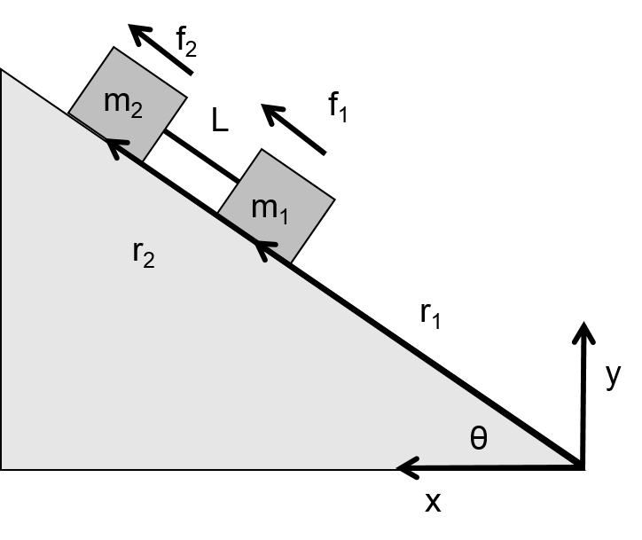
Determine the equation of motion for two blocks of mass, \(m_1\) and \(m_2\), that are connected by a mass-less rod of length, \(L\), and are sliding with friction down an inclined slope of angle \(\theta\). The friction forces have magnitudes \(f_1\) and \(f_2\).
Figure 4.2Two connected block sliding with friction
We start by identifying that there is only 1 degree of freedom, and we choose the variable \(r=r_1\) as the generalized coordinate (the distance from the first block to the origin in Figure 4.2). The coordinate transformations are thus:
again, we recover Newton’s Second Law. The use of generalized coordinates makes it more obvious that this can be treated as a single system of mass \(m_1+m_2\) and total non-monogenic force \(f_1+f_2\).
The connection to variational calculus and the use of auxiliary constraints
It should be clear now that systems can be described by the Lagrangian, \(L=T-V\). Although we have shown abundantly that this is equivalent to D’Alembert’s Principle (which itself is equivalent to Newton’s Second Law), the approach is conceptually very different. The Lagrangian is only constructed using scalar quantities that are related to energy. The concept of a force is no longer fundamental to describing a system, and describing the energy is the fundamental concept. Generalized forces are in general not in the same units as those in Newton’s Second Law, and, as we saw in the previous chapter, can also be related to torques.
In the case that all forces are monogenic, and the system is holonomic, the equations of motion, \(q_i(t)\) for \(n\) degrees of freedom can be written as the requirement that the action, \(S\), is stationary:
which are called the “Euler-Lagrange” equations from variational calculus. In the case where they are applied to mechanics, we often call them “Lagrange’s equations of motion”.
The requirement that the system be holonomic can be relaxed somewhat. We required that the system be holonomic so that the generalized coordinates can be varied independently. We however know from the calculus of variations that we can include “auxiliary conditions” between the generalized coordinates using Lagrange multipliers and treat the system as being holonomic. More precisely, if we have \(k\) equations of the form \(f(q_1,\dots q_n)=0\), the Lagrangian can be modified to be:
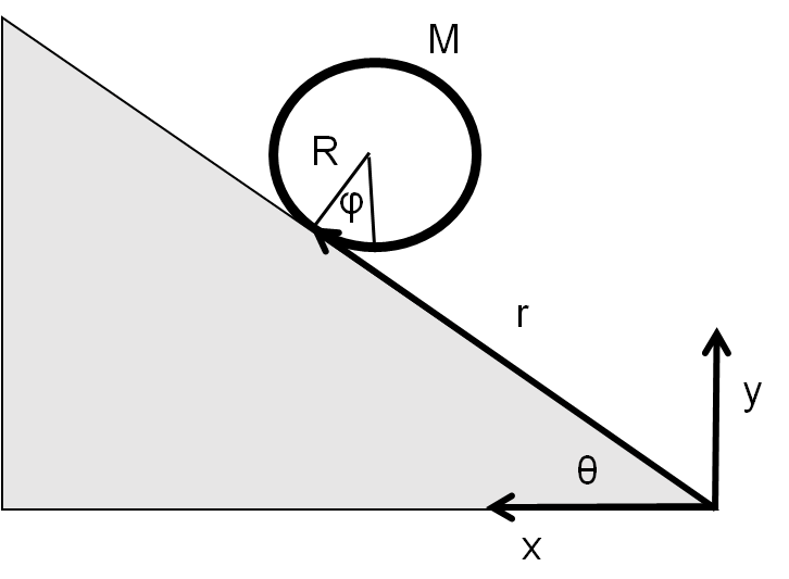
Determine the equations of motion for a hoop of mass \(M\) and radius \(R\) as is rolls without slipping down an incline of angle \(\theta\). Use the method of Lagrange multipliers to handle the constraint of rolling without slipping.
Figure 4.3Hoop of mass, \(M\) and radius \(R\) rolling without slipping down an incline.
Although this situation has only 1 degree of freedom (we could choose \(r\) or \(\phi\)), we will use both \(r\) and \(\phi\) to describe the hoop and introduce an equation of constraint. Although the constraint is non-holonomic (rolling without slipping is a condition on the velocity of the point of contact), in 1 dimension it can be integrated to be holonomic:
where \(k\) is a constant offset between the height of the center of mass and the point of contact of the hoop and incline. Since \(k\) will vanish from the Euler-Lagrange equations, we will neglect it.
where it is clear that \(\lambda\) has the dimensions of force. Additionally, differentiating the equation of constraint twice with respect to time, we have:
Re-moving the explicit dependence on \(\lambda\) from the equations of motion:
\begin{align*}
M\ddot{r}&=-\frac{1}{2}Mg\sin{\theta}\\
MR^2\ddot{\phi}&=-\frac{1}{2}Mg\sin{\theta} R
\end{align*}
Note that \(\lambda\) can be associated with the force that makes the hoop rotate (the contact force that is tangent to the hoop). The last equation is the rotational equivalent of Newton’s Second Law, using torque, \(\tau\), and the angular acceleration, \(\alpha\), (\(I\alpha=\tau\)). The components of the monogenic forces corresponding to \(\lambda\) are:
Determine the equations of motion for a hoop of mass \(M\) and radius \(R\) as is rolls without slipping down an incline of angle \(\theta\). Use the method of Lagrange multipliers to handle the constraint of rolling without slipping and that of the hoop being constrained to the incline.
We repeat the previous problem, but now use three coordinates to describe the hoop. We use \(\phi\), the rotation angle, in addition to \(x\) and \(y\) to describe the position of the point of contact between the hoop and the incline. Using the fact that \(y=r\sin{\theta}\) to include the rolling without slipping condition from the previous example, we have:
The potential energy is given by that of the center of mass:
\begin{align*}
V&=Mgy
\end{align*}
where, again, we do not need to worry that the point of contact of the hoop is different by a constant offset from the position of the center of mass. The Lagrangian and modified Lagrangian (with two constraints) are thus:
These equations are equivalent to the ones in the previous example. Again, \(\lambda_2\) is associated with the force tangent to the hoop that makes the hoop turn. \(\lambda_1\) is related to the normal force on the incline (it is maximal at \(\theta=0\) and vanishes at \(\theta=\frac{\pi}{2}\)). The components of the monogenic forces corresponding to \(\lambda_1\) and \(\lambda_2\) are:
The only one that is really straightforward to interpret is \(Q_{2\phi}\), corresponding to the torque that makes the hoop rotate down the incline.
It should become clear to the reader that the concept of force is getting more obscure as we arrive at a more general description of classical mechanics in the analytic framework. It is important to understand that issues of constraint are often related to the forces from vectorial mechanics, although it is generally not necessary to use the concept of force to describe a system.
As we generalize further, we will also restrict ourselves to systems that are holonomic and monogenic. This is in fact a rather good approximation to nature. Most non-monogenic forces (for example, friction) arise from the fact that we limit ourselves to considering a restricted system (for example, we consider only a block sliding with friction). If we consider a system as a whole (for example, the block and the incline), then most forces become workless “internal” forces of constraint. Indeed, if we consider the Universe as a whole, then only four fundamental forces are responsible for all interactions (gravity, electromagnetic, strong nuclear, weak nuclear). Furthermore, in the classical macroscopic world, only the electromagntic and gravitational forces are of consideration, and these are both monogenic.