3.1 Virtual work

Virtual work, \(\delta W_i\) is the work done by a force, \(\vec{F}_i\) given a “reversible virtual displacement” that is in harmony with the given constraints, \(\delta\vec{r}_i\):

A reversible displacement is one where \(\delta\vec{r}_i\) can be replaced with \(-\delta\vec{r}_i\) without violating any of the constraints \(\delta\vec{r}_i\) is the variation of the position vector where the force is applied. By definition, a virtual displacement that is parallel to a normal force is not reversible.

Principal of virtual work and static equilibrium

The principle of virtual work states that for a static equilibrium, the sum of virtual work done by all forces is equal to zero.

We can divide this up into “external forces” (such as gravity, electric fields), \(\vec{F}^E_i\), and “internal forces” (such as tension in a rod, normal reaction forces), \(\vec{F}^I_j\).

Typically, the internal forces are related to constraints. “Workless constraints” are those that lead to forces that do no virtual work.

Example 3-1

The tension force in a rigid rod that holds two masses together is workless

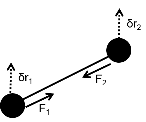
The tension forces on each mass are equal and opposite (Newton’s third law):

\begin{align*} \vec{F}_1=-\vec{F}_2 \end{align*}

Furthermore, the constraint that the rods be fixed relative to each other requires that their virtual displacement be the same:

\begin{align*} \left|\vec{r}_2-\vec{r}_1\right|=l\nonumber\\ \delta \left|\vec{r}_2-\vec{r}_1\right|=\delta l=0\nonumber\\ \therefore \delta\vec{r}_1=\delta \vec{r}_2 \end{align*}

Thus, the virtual work done by the internal forces in this case is zero:

\begin{align*} \sum\vec{F}^I_j\cdot\delta\vec{r}_j&=\vec{F}_1\cdot\delta\vec{r}_1+\vec{F}_2\cdot\delta\vec{r}_2\nonumber\\ &=\vec{F}_1\cdot\delta\vec{r}_1-\vec{F}_1\cdot\delta\vec{r}_1=0 \end{align*}

Example 3-2

The normal force on a frictionless surface is workless

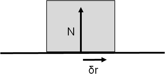
If the block is constrained to slide on the surface, the normal force is perpendicular to \(\delta \vec{r}\) and thus does no virtual work. \(\delta \vec{r}\) must be parallel to the contact surface, since it would not be reversible otherwise.

In the case of workless constraints, the total virtual work is given by the work of the external forces. It is generally true (although difficult to prove) that most constraint forces are workless and can be ignored.

For static equilibrium, the “Principal of Virtual Work” states that the total virtual work (which is done by external forces) must be zero:

This is in contrast to the vectorial approach with requires the sum of all forces (external and internal) to be zero.

Generalized forces

We continue by ignoring the internal forces and consider the virtual work done by N external forces:

If we have \(n\) degrees of freedom, we can re-write this in terms of the generalized coordinates (where holonomic constraints are used to reduce the number of coordinates, and the coordinates are thus all independent):

where we have introduced the components, \(Q_j\), of the “generalized force” which do not necessarily have the dimensions of force:

The total work is thus the scalar product of the generalized force, \(\vec Q\), and a virtual displacement vector, \(\delta \vec q\), in configuration space:

If any displacement is allowed in configuration space, \(\delta \vec{q}\), then all components of the generalized force must be zero for static equilibrium. In a holonomic system, where all coordinates are independent of each other, \(\delta {q}_i\) all correspond to allowed displacements and the generalized force components are therefore zero. Another way to picture this is that, given generalized coordinates \(q_j\), the generalized force \(Q_j\) is the force that does work \(Q_j \delta q_j\) when the system is displaced in the direction \(\delta q_j\). Since \(q_j\) is not necessarily a cartesian coordinate (it could be an angle), \(Q_j\) does not necessarily have the units of force.

Using the Principal of Virtual Work to solve statics problems

We proceed with a few examples for solving statics problems using the principal of virtual work. The general procedure will be as follows:

1. Identify the number of degrees of freedom and choose generalized coordinates

2. Identify the forces that can perform virtual work (forces acting at points where a virtual displacement is possible given the constraints, and forces that are not perpendicular to the allowable virtual displacements)

3. Write the position vectors of the points where the forces are applied in terms of the generalized coordinates. Then, take the variations in those vectors to obtain the \(\delta \vec r_i\)

4. Write out the virtual work and set it to zero

5. (Alternatively) Evaluate the components of the generalized force and set them equal to zero

Example 3-3

What is the magnitude, \(F\), of the horizontal force required to maintain a pivoting bar (restricted to pivot in a plane) of mass \(m\), length \(2L\), and negligible diameter (see Figure 3.3) at an angle \(\theta\)?

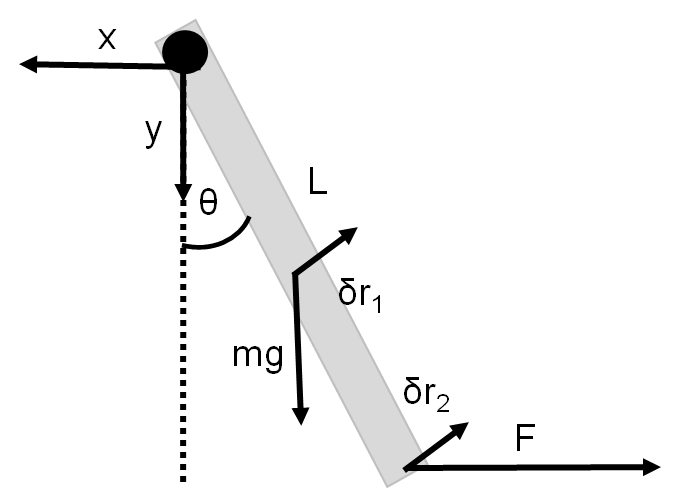
This is a rigid body, so in principle there are 6 degrees of freedom. If we choose a coordinate system at the pivot point, we can describe the position of the bar by the cartesian coordinates of the pivoting end of the bar, and 3 angles to describe the rotation of the bar about the 3 axes. However, we have the following constraints:

\begin{align*} x&=0\nonumber\\ y&=0\nonumber\\ z&=0\nonumber\\ \theta_x &=0\nonumber\\ \theta_y &=0\nonumber\\ \end{align*}

we are thus left with 1 degree of freedom. We choose \(\theta=\theta_z\) as the one generalized coordinate. Next we consider the virtual work of the forces that can perform non-zero virtual work (the forces at the pivot point cannot perform any virtual work, as the pivot point cannot be moved; its virtual displacement would not be in harmony with the constraints). We have gravity and \(F\) that do virtual work:

\begin{align*} \delta W = mg\hat y\cdot\delta\vec{r}_1-F\hat x\cdot\delta\vec{r}_2 \end{align*}

The virtual displacement vectors must be consistent with the kinematic constraints, that is, they are perpendicular to the rod (and the constraints require that \(\delta\vec{r}_1\) and \(\delta\vec{r}_2\) point in the same direction). We can write the position vectors for the points where the forces are applied and take their variation with respect to \(\theta\):

\begin{align*} \vec{r}_1=L(-\sin{\theta}\hat{x}+\cos{\theta}\hat{y})\\ \vec{r}_2=2L(-\sin{\theta}\hat{x}+\cos{\theta}\hat{y})\\ \therefore \delta\vec{r}_1=L(-\cos{\theta}\hat{x}-\sin{\theta}\hat{y})\delta\theta\\ \therefore \delta\vec{r}_2=2L(-\cos{\theta}\hat{x}-\sin{\theta}\hat{y})\delta\theta\\ \end{align*}

Thus:

\begin{align*} \sum_{i=1}^N\delta W_i = -mgL\sin{\theta}\delta\theta+ 2LF\cos{\theta}\delta\theta \end{align*}

Setting the virtual work to zero, we get the same answer as you would using introductory mechanics techniques (e.g. torques):

\begin{align*} F=\frac{1}{2}mg\tan{\theta} \end{align*}

Let’s calculate the generalized force:

\begin{align*} Q_j&\equiv \sum_{i=1}^N\vec{F}_i\cdot\frac{\partial\vec{r}_i}{\partial q_j}\nonumber\\ \end{align*}

Note that \(N=2\) and there is only 1 \(q_j\), namely \(\theta\). If we write the vectors in the xy coordinates, we can evaluate the partial derivatives:

\begin{align*} \frac{\partial\vec{r}_i}{\partial \theta}&=L(-\cos{\theta}\hat{x}-\sin{\theta}\hat{y}) \\ \frac{\partial\vec{r}_2}{\partial \theta}&=2L(-\cos{\theta}\hat{x}-\sin{\theta}\hat{y})\\ \end{align*}

The generalized force is then given by:

\begin{align*} Q_\theta&=m\vec{g}\cdot\left(L(-\cos{\theta}\hat{x}-\sin{\theta}\hat{y})\right)+\vec{F}\cdot\left(2L(-\cos{\theta}\hat{x}-\sin{\theta}\hat{y})\right)\\ &=-Lmg\sin{\theta}+2LF\cos{\theta} \end{align*}

And you may recognize that the generalized force in the \(\theta\) direction is the total torque! The requirement that the generalized force be zero is the same as requiring that the sum of the torques are zero.

Example 3-4

Find the magnitude of the force, \(F\), required to keep the system in equilibrium from Figure 3.4 at an angle \(\theta\). The blocks of mass \(m\) slide with no friction and are held by a mass-less rigid rod of length, \(L\). Their dimensions are negligible.

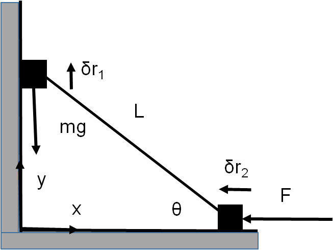
Since we have 2 particles, we have 6 possible degrees of freedom. However, each particle is constrained to move along only 1 axis, thus reducing the number of degrees of freedom by 4. Furthermore, the particles are connected by a rigid rod, which further reduces the number of degrees or freedom by 1. There is only 1 degree of freedom, and we choose \(\theta\) as our generalized coordinates. The constraint equations are:

\begin{align*} x_1&=0\nonumber\\ z_1&=0\nonumber\\ y_2&=0\nonumber\\ z_2&=0\nonumber\\ y_1^2+x_2^2&=L^2\\ \end{align*}

We have 2 forces that can perform virtual work: gravity on particle 1 and \(F\) on particle 2. Gravity on particle 2 cannot perform virtual work as it is perpendicular to the allowable virtual displacements of particle 2.

\begin{align*} \sum_{i=1}^N\delta W_i &= m\vec{g}\cdot\delta\vec{r}_1+\vec{F}\cdot\delta\vec{r}_2\\ \end{align*}

Writing the position vectors for the points where the forces are applied and calculating their variation with respect to \(\theta\):

\begin{align*} \vec{r}_1&=0\hat{x}+L\sin{\theta}\hat{y}\\ \vec{r}_2&=L\cos{\theta}\hat{x}+0\hat{y}\\ \delta\vec{r}_1&=L\cos{\theta}\delta\theta\hat{y}\\ \delta\vec{r}_2&=-L\sin{\theta}\delta\theta\hat{x} \\ \end{align*}

The virtual work is then:

\begin{align*} \sum_{i=1}^N\delta W_i &= -mgL\cos{\theta}\delta \theta + FL\sin{\theta}\delta \theta=0 \\ \therefore F&=mg\cot{\theta} \end{align*}

It is straightforward to show that the generalized force is equal to the sum of the torques:

\begin{align*} Q_\theta &= -mgL\cos{\theta}+FL\sin{\theta}\\ \end{align*}

Example 3-5

Find the value of \(\theta\) for the two blocks in Figure 3.5 to be in equilibrium. The blocks of mass \(m\) and \(2m\) are sitting on a frictionless sphere of radius \(R\) and are connected by a mass-less inextensible string of length \(L\).

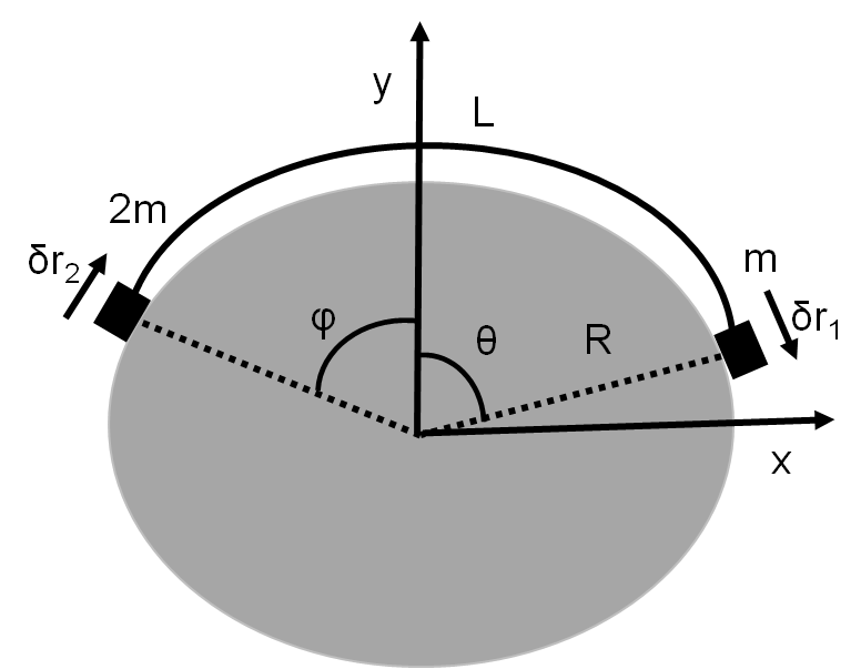
There is only 1 degree of freedom, and we choose \(\theta\) as the generalized coordinate. The angles \(\phi\) and \(\theta\) are related by:

\begin{align*} \phi=\frac{L}{R}-\theta\\ \therefore \delta\phi = -\delta \theta \end{align*}

By writing the position vectors for each particle (where the forces of gravity are applied), we can get their virtual displacements:

\begin{align*} \vec{r}_1&=R(\sin{\theta}\hat{x}+\cos{\theta}\hat{y})\\ \vec{r}_2&=R(-\sin{\phi}\hat{x}+\cos{\phi}\hat{y})\\ \delta\vec{r}_1&=R(\cos{\theta}\hat{x}-\sin{\theta}\hat{y})\delta\theta\\ \delta\vec{r}_2&=R(-\cos{\phi}\hat{x}-\sin{\phi}\hat{y})\delta\phi\\ &=R(\cos{\phi}\hat{x}+\sin{\phi}\hat{y})\delta\theta\\ \end{align*}

The virtual work is then given by the weights multiplied by the y-components:

\begin{align*} \sum_{i=1}^N\delta W_i&=mgR\sin{\theta}\delta\theta-2mgR\sin{\phi}\delta\theta\\ &=mgR(\sin{\theta}-2\sin{(\frac{L}{R}-\theta}))\delta\theta=0\\ &=\sin{\theta}-2(\sin{\frac{L}{R}}\cos{\theta}-\cos{\frac{L}{R}}\sin{\theta})\\ &=\tan{\theta}-2(\sin{\frac{L}{R}}-\cos{\frac{L}{R}}\tan{\theta})\\ \therefore\tan{\theta}&=\frac{2\sin{\frac{L}{R}}}{(1+2\cos{\frac{L}{R}})} \end{align*}

where we used the formula \(\sin{(\alpha-\beta)}=\sin\alpha\cos\beta -\cos\alpha\sin\beta\). The generalized force is:

\begin{align*} Q_\theta=mgR\left(\tan{\theta}((1+2\cos{\frac{L}{R}}))-2 \sin{\frac{L}{R}} \right) \end{align*}