1.2 Definitions and notation

Particle, position, velocity, acceleration

We will define a “particle” to be a point-like object with a mass. The location in space of such a particle is described by a position vector, \(\vec{r}(t)\), that can change as a function of time. The components of the position vector are the “coordinates” of the particle. The rate of change of the position vector is called “velocity” (and that of velocity, “acceleration”). If one knows the values of the position and velocity vectors at some instant in time, the whole “path” of the particle (backwards and forwards in time and space) can be deduced. The equations that relate position, velocity, and acceleration are called “equations of motion”. Newton’s second law gives the equation of motion for \(\vec{r}(t)\) in differential form:

\begin{align} \vec{F}&=m\vec{a}=m\frac{d^2}{dt^2}\vec{r}=m\ddot{\vec{r}}\\ \ddot{\vec{r}}&=\frac{1}{m}\vec{F} \tag{1.2}\end{align}

where we have introduced the use of “dots” to signify derivatives with respect to time:

\begin{align} \vec{F}&=m\vec{a}=m\frac{d^2}{dt^2}\vec{r}=m\ddot{\vec{r}}\\ \dot{x}&\equiv\frac{d}{dt}x\\ \ddot{x}&\equiv\frac{d^2}{dt^2}x\end{align}

Rigid body

A “rigid body” is an object made from many particles that are fixed in position relative to each other. The rigid body can thus be treated without knowing the specifics of the particles that make it up. Often, it is sufficient to describe a rigid body by the position of its center of mass, its angles of rotation about three axes, its total mass, and its moment of inertia tensor.

Degrees of freedom

The “number of degrees of freedom” is the number of scalar quantities that are required to specify the state of a system. For a particle in three dimensional space, one requires 3 coordinates to specify the location of a particle. For a rigid object, one requires 6 degrees of freedom (3 coordinates of the center of mass and 3 rotation angles).

System

A “system” is an ensemble of particles and rigid bodies that one wants to describe. A system will generally have 3N+6M degrees of freedom, if there are N particles and M rigid bodies.

Constraints

When there are “constraints” applied to the coordinates of the particles, the number of degrees of freedom is reduced. For example, if 2 particles are connected by a rigid mass-less bar of length, \(l\), the number of degrees of freedom is 5. The constraint of a rigid bar can be written as 1 equation of constraint, requiring that the distance between the two particles remain constant.

\begin{align} |\vec{r_1}-\vec{r_2}|^2=(x_1-x_2)^2+(y_1-y_2)^2+(z_1-z_2)^2=l^2\\ \therefore l^2-(x_1-x_2)^2+(y_1-y_2)^2+(z_1-z_2)^2=0 \tag{1.4}\end{align}

we call this a “constraint” equation. In general, the number of degrees of freedom is reduced by the number of constraint equations that exist. For two masses constrained by a bar, we have 5 degrees of freedom. This makes sense; we can completely specify the position of the two masses by the 3 coordinates of the first mass and 2 angles that specify the rotation of the bar.

Example 1-2

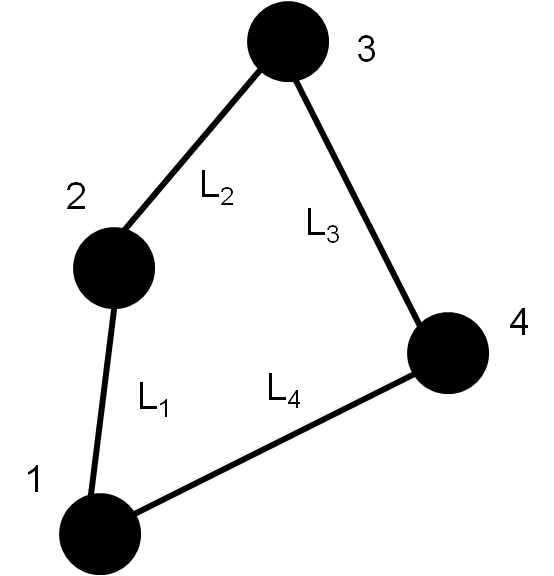
How many degrees of freedom are required to describe a system of 4 particles connected by 4 rigid massless rods? Write out the constraint equations. What if the particles are constrained to the xy-plane?

4 Masses And Rod — Figure 1.2Four particles connected by rods

Without constraints, the system would be described by 12 degrees of freedom (4 particles with 3 coordinates). Each rod \(k\) introduces an equation of the form:

\begin{align*} (x_i-x_j)^2+(y_i-y_j)^2+(z_i-z_j)^2=l_k^2 \end{align*}

between the coordinates of particle \(i\) and particle \(j\). There are thus \(12-4=8\) degrees of freedom. If the particles are constrained to the xy-plane, we can introduce 4 more constraint equations of the form:

\begin{align*} z_i=0\text{ (i=1,2,3,4)} \end{align*}

giving us 4 degrees of freedom. Equivalently, we could start in a two-dimensional space, where the un-constrained system would have 8 degrees of freedom, and the 4 constraints from the rods would also bring this down to 4.

Types of constraints

Different types of constraints have different properties (and names).

Holonomic

Constraint equations that can be written using the coordinates of the particles in the system are called “holonomic”. The constraint equation with two masses held by a rigid bar is an example of a holonomic constraint (see eqn. 1.4). A holonomic constraint can depend on time.

Example 1-3

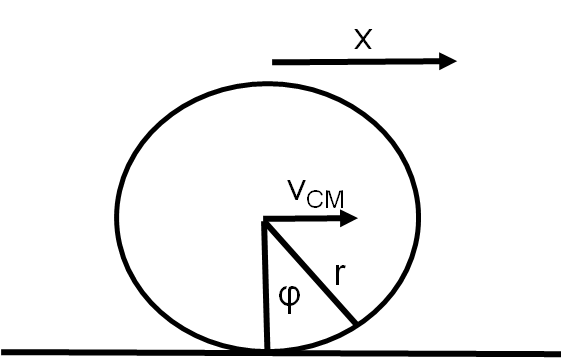
Rolling without slipping in 1D. Write out the constraint for a disk of radius \(r\) to roll without slipping along the x-axis.

Rolling1 D — Figure 1.3A disk rolling without slipping

The constraint for rolling without slipping is that the instantaneous velocity of the point of contact is zero. The velocity of the point of contact is in the x-direction and has a magnitude:

\begin{align*} v_{CM}-r\dot{\phi}&=0\nonumber\\ \therefore v_{CM}&=r\dot{\phi} \end{align*}

Using the generalized coordinate \(x\) to describe the position of the center of mass of the disk:

\begin{align*} v_{CM}&=\frac{dx}{dt}\nonumber\\ \therefore \frac{dx}{dt}=r\frac{d\phi}{dt} \end{align*}

which is not a holonomic constraint. However, we can integrate it to get a holonomic constraint:

\begin{align*} dx=rd\phi\nonumber\\ \therefore x=r\phi \end{align*}

Non-holonomic

Non-holonomic constraint equations cannot be written only in terms of the coordinates, or contain inequalities. For example, the constraint of “rolling without slipping” is a constraint on the instantaneous velocity of the point of contact. The equation is expressed in terms of the velocity rather than the position coordinates (it can be integrated in 1 dimension to get a holonomic constraint, but this does not generalize to 2-dimensions). Another type of non-holonomic constraints are those that contain inequalities such as particles that are constrained to move within a volume (the constraint is on the position vectors, but it is expressed as an inequality). In general, it is difficult to deal with non-holonomic constraints.

Example 1-4

The constraint equation for particles constrained to be inside of a sphere of radius \(R\):

If the origin is at the center of the sphere, each particle \(i\) provides a constraint equation of the form:

\begin{align*} x_i^2+y_i^2+z_i^2<R^2 \end{align*}

Example 1-5

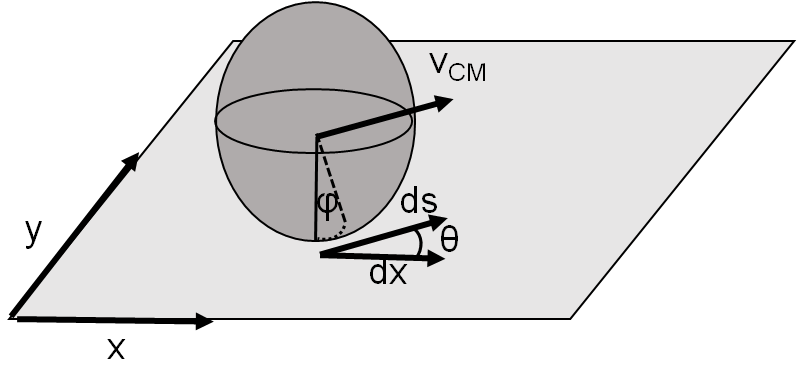
Rolling without slipping in 2D. Write out the constraint for a sphere of radius \(r\) to roll without slipping in the xy-plane

Rolling2 D — Figure 1.4A sphere rolling without slipping

Again, the constraint for rolling without slipping is that the instantaneous velocity of the point of contact is zero.

\begin{align*} \frac{ds}{dt}-r\dot{\phi}&=0\nonumber\\ \frac{ds}{dt}&=r\frac{d\phi}{dt}\nonumber\\ ds&=r d\phi \end{align*}

where \(ds\) is the displacement of the center of mass, and \(d\phi\) is the infinitesimal angle around the current axis of rotation (which is perpendicular to \(d\vec{s}\)). If the (instantaneous) direction of the ball rolling with respect to the x-axis is given by \(\theta\). We have:

\begin{align*} dx&=ds\cos{\theta} =r\cos{\theta}d\phi\nonumber\\ dy&=ds\sin{\theta} =r\sin{\theta}d\phi\nonumber\\ \end{align*}

which is not a holonomic constraint. \(\theta\) depends on time (we have no constraint on which direction the ball is allowed to roll), thus, we cannot simply integrate these equations, and they remain in their differential form.

Sceleronomous

A sceleronomous constraint does not depend explicitly on time (the partial derivative with respect to time is zero).

Rheonomous

A rheonomous contraint depends (explicitly) on time (partial derivative with respect to time is non-zero).

Generalized coordinates

In general, one has the freedom to choose the coordinate system (Cartesian, polar, something more exotic) to describe a system. If we have a system with \(N\) particles and \(k\) holonomic constraints, there will be \(3N\) coordinates, but only \(3N-k\) of them will be independent (the number of degrees of freedom).

It is often useful to restrict the number of coordinates to describe a system so that there are only as many coordinates as there are degrees of freedom. These coordinates are called “generalized coordinates”, and often denoted as the set \(\{q_1,q_2,q_3,\dots,q_{3N-k}\}\). Their time derivatives are called “generalized velocities” \(\{\dot{q_1},\dot{q_2},\dot{q_3},\dots,\dot{q}_{3N-k}\}\). The generalized coordinates should not necessarily be thought of as a set of coordinates in space (like Cartesian or Polar); rather, a set of numbers that describes the state of the system.

Using generalized coordinates, one does not need to think in terms of the coordinates of each particle in the system. That is, the generalized coordinates may not be the position of specific particles, but rather numbers that can describe the ensemble of particles. The system is entirely described by the generalized coordinates. There will exist “transformation equations” to convert the generalized coordinates back to the coordinates of the individual particles in the system:

\begin{align} x_1&=x_1(q_1,q_2,q_3,\dots,q_{3N-k},t)\\ y_1&=y_1(q_1,q_2,q_3,\dots,q_{3N-k},t)\\ z_1&=z_1(q_1,q_2,q_3,\dots,q_{3N-k},t)\\ &\dots\\ x_N&=x_N(q_1,q_2,q_3,\dots,q_{3N-k},t)\\ y_N&=y_N(q_1,q_2,q_3,\dots,q_{3N-k},t)\\ z_N&=z_N(q_1,q_2,q_3,\dots,q_{3N-k},t)\end{align}

The generalized coordinates could have different units than length and could, in general, be quite abstract. The transformation equations to the generalized coordinates can depend on time. Similarly, the generalized velocities (and accelerations), can also be obtained from the transformation equations:

\begin{align} \dot{x}_1&=\frac{\partial x_1}{\partial q_1}\dot{q}_1+\dots+\frac{\partial x_1}{\partial q_{3N-k}}\dot{q}_{3N-k}+\frac{\partial x_1}{\partial t}\\ &\dots\\ \dot{z}_N&=\frac{\partial z_N}{\partial q_1}\dot{q}_1+\dots+\frac{\partial z_N}{\partial q_{3N-k}}\dot{q}_{3N-k}+\frac{\partial z_N}{\partial t} \end{align}

The partial derivative with respect to time comes from writing \(dx = \frac{\partial x_1}{\partial q_1}dq_1+\dots +\frac{\partial x_1}{\partial t} dt\) and then dividing out by \(dt\) to get \(\dot{x}\) on the left hand side.

Example 1-6

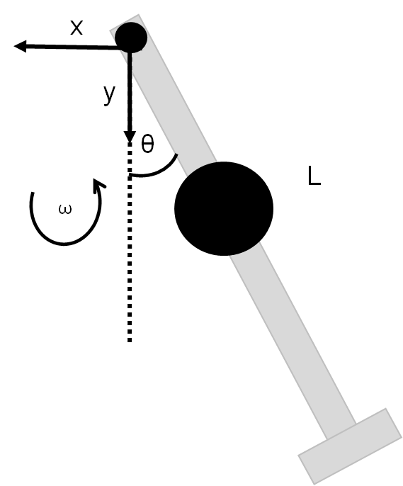
Write out generalized coordinates to describe the motion of a bead of mass \(m\) that is constrained to slide along a mass-less rod of length, \(L\), that is rotating at a constant angular frequency \(\omega\) in the vertical plane about its pivot point (Figure 1.5). Write out the constraint equations in the form \(f_i(x_1,\dots ,x_n)=0\). Write out the generalized velocities.

Bead On Rod — Figure 1.5Bead that can slide on a rotating rod.

Since we are describing a particle, we have 3 degrees of freedom. However, the bead is constrained to be in the horizontal plane (\(z=0\)) as well as being on the rod. These two constraints thus reduce the number of degrees of freedom to 1. We can choose to describe the particle by its distance from the pivot point of the rod, \(r\). We thus have:

\begin{align*} x(t) &=-r\sin{\omega t}\nonumber\\ y(t) &=r\cos{\omega t} \end{align*}

The constraint equations are:

\begin{align*} z&=0\nonumber\\ x+y\tan{\omega t}&=0 \end{align*}

There is an additional non-holonomic constraint, since the rod has a stop at the end. This does not reduce the number of degrees of freedom:

\begin{align*} x^2+y^2-L^2\leq 0 \end{align*}

The generalized velocity transformations are:

\begin{align*} \dot{x} &=-\dot{r}\sin{\omega t}-r\omega\cos{\omega t}\\ \dot{y} &=\dot{r}\cos{\omega t}-r\omega\sin{\omega t} \end{align*}

Configuration space

The \(n\) generalized coordinates corresponding to the \(n\) degrees of freedom of a system can be thought of in terms of an n-dimensional Euclidean space called “configuration space”. As the system evolves through time, one can relate this to a path in configuration space. The equations of motion dictate that path. Note that the initial conditions of a system will dictate which path it takes in coordinate space based on the equations of motion. For example, a cannon ball has the same equations of motion regardless of the inclination of the cannon its initial velocity as it exits the cannon. However, depending on the initial conditions of its position and velocity, the cannon ball will trace different trajectories (paths in configuration space).