1.1 Analytic and vector mechanics

In introductory physics, one learns to describe the time evolution of a system using Newton’s second law of motion. This approach to mechanics is called “vector mechanics”. Newton’s second law:

\begin{align} \vec{F}=m\vec{a} \tag{1.1}\end{align}

is a vector equation that is true for each component of the vectors for force and acceleration.

By contrast, in “analytic mechanics”, the formalism is developed to describe the time-evolution of a system using a single equation involving only scalar quantities. The approach will be seen to be equivalent to the vector mechanics approach. The vector mechanics formalism generally suffers from limitations that make it difficult to apply in complicated situations. For example, the vector equations are not straightforward in non-Cartesian coordinate systems, which may be more suited for certain problems (motion on the surface of a sphere, orbital motion, etc.).

In general, a “theory” of classical mechanics should be able to describe the future and past of a system, given knowledge of its current state and the forces involved. We will see that it is sufficient to describe the current state of a system by specifying the positions of all of the particles that are involved. Furthermore, given the particular forces (or potential energies involved), knowing the positions and velocities of all particles is sufficient in order to describe the entire history (past and future) of the system. The analytic treatment of mechanics is formulated using the positions and velocities of the particles involved (as opposed to the vectorial approach that deals with accelerations).

Example 1-1

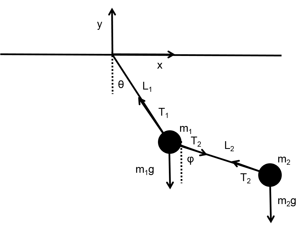
The Compound Pendulum is a typical example of a simple system that is awkward to describe using vectorial analysis, but straightforward using analytic mechanics.

Compound Penduluum — Figure 1.1Vectorial analysis of the compound pendulum

In order to describe the motion of the two masses as a function of time, we start by defining an origin, and label the coordinates of mass \(i\) with \(x_i\) and \(y_i\). We wish to find the functions \(x_i(t)\) and \(y_i(t)\) given initial conditions on the positions and velocities of the masses. We have 6 unknowns (the accelerations in \(x\) and \(y\) of the two masses, and the two string tensions).

Newton’s second law gives, in vectorial form:

\begin{align*} m_1\vec{a}_1&=\vec{T}_1+\vec{T}_2+m_1\vec{g}\\ m_2\vec{a}_2&=\vec{T}_2+m_2\vec{g}\\ \end{align*}

Writing this out, component by component, we have:

\begin{align*} m_1 \ddot x_1&=T_2\sin\phi-T_1\sin\theta\\ m_1 \ddot y_1&=T_1\cos\theta-T_2\cos\phi-m_1g\\ m_2 \ddot x_2&=-T_2\sin\phi\\ m_2 \ddot y_2&=T2\cos\phi-m_2g \end{align*}

where we have introduced the notation of \(\ddot x \equiv \frac{d^2x}{dt^2}\) for the accelerations (a dot on top of a variable represents a time derivative, two dots represent a second order derivative). It may appear that we have 8 unknowns (the \(x_i\), \(y_i\), \(T_i\) and the two angles). However, due to the constraints of the masses being attached to massless rods of the pendulum, the position coordinates are all related and only two of them are independent. One can choose the two angles to be the independent variables, since they are given by the \(x_i\) and \(y_i\):

\begin{align*} x_1&=L_1\sin\theta\\ y_1&=-L_1\cos\theta\\ x_2&=x_1+L_2\sin\phi\\ y_2&=y_1-L_2\cos\phi \end{align*}

One can then replace the accelerations using the Chain Rule to re-express the accelerations in terms of \(\theta\) and \(\phi\):

\begin{align*} \dot x_1&=\frac{d}{dt}L_1\sin\theta=L_1\cos\theta\dot\theta\\ \ddot x_1&=\frac{d}{dt}L_1\cos\theta\dot\theta=L_1(\cos\theta\ddot\theta-\sin\theta\dot\theta^2) \end{align*}

and eliminate all the \(x_i\) and \(y_i\). One is then left with four equations and four unknowns (\(\ddot\theta\), \(\ddot \phi\), \(T_1\), \(T_2\)). The equations for the angular acceleration form a set of coupled second order ODEs that can be solved numerically.

One could alternatively choose to eliminate the angles and the \(y_i\), since the \(y_i\) can be written in terms of the \(x_i\):

\begin{align*} y_1&=-\sqrt{L_1^2-x_1^2}\\ y_2&=y_1-\sqrt{L_2^2-(x_2-x_1)^2)} \end{align*}

and one would then use the Chain Rule to re-express the \(\ddot y_i\) in terms of the \(\ddot x_i\).